Differentiable DSP

Lecture 10 · Keep the structure, learn the parameters

Prof. Dr.-Ing. Sebastian J. Schlecht

Where we are

One question, asked of every method

Block	Representation	Generator
Filters and effects	LTI and time-varying systems	hand-designed
Classical synthesis	samples, partials, modes, physical state	hand-designed
DDSP	the same structured models	parameters learned
Reverberation	a recursive dynamical system	hand-designed, fittable
Diffusion	a learned representation	learned

 

The four questions

1. How is the sound represented?
2. What are the controllable parameters?
3. What structure is built in?
4. What is fixed by design, and what is learned?

Every lecture so far ended with a match step that we did by ear: pick a cutoff, an FM index, a pluck position until it sounds right. Today that step becomes an optimization.

Listen

Three matches, done by gradient descent

A room (next lecture)

target
FDN, start
FDN, fitted

 

A guitar note (lecture 9)

target
modal string, by ear
modal string, fitted

 

An amplifier, on a recording it never saw

clean input
the amp
model, fitted

Listen first

In each column, the model’s structure was fixed in advance. What exactly was learned? And is a model that sounds right necessarily a model with the right parameters?

The idea

The match step, automated

\[\hat{\theta} = \arg\min_\theta\; L\big(f_\theta(u),\ y_\text{target}\big), \qquad \theta \leftarrow \theta - \eta\,\frac{\partial L}{\partial \theta}\]

Differentiable DSP

Write the synthesizer or effect in an automatic-differentiation framework (PyTorch, JAX), so the gradient of a loss flows back through every filter, oscillator and delay into its parameters. The structure stays hand-designed; the numbers are learned.

Black box, white box, grey box

Black box

A network learns the input–output behavior from data. Standard today for amps and pedals (recurrent networks, Wright et al. 2019; the open Neural Amp Modeler). No knobs inside.

 

White box

Known topology and equations, translated into a simulation: lectures 7 to 9 and 11, and Max’s wave digital filters for circuits. Every parameter has a meaning, but someone has to measure it.

 

Grey box

Keep the structure, learn the parameters, or learn only the parts nobody can write down (a body filter, a nonlinearity). DDSP lives here.

The grey box keeps what a musician needs: the fitted model is still a string, a reverb, an amp, with the same knobs as before.

DDSP (Engel et al., 2020)

 

• lecture 7’s additive synthesis and subtractive noise, a reverb (lecture 11)
• the pitch comes from a pitch tracker, not from gradient descent
• a small network predicts, every few ms, the harmonic amplitudes and the noise filter
• trained with a multi-scale spectral loss on one instrument, e.g. 13 minutes of violin

Timbre transfer: sing into a model trained on violin, and the analysis (f₀, loudness) drives a violin. The representation is the control.

Also differentiable: wavetables (Shan et al. 2022), FM (DDX7, Caspe et al. 2022), IIR filters and parametric EQs, FDNs (Dal Santo et al. 2023), whole effect chains for style transfer (Steinmetz et al. 2022). Hayes et al. (2024) review the field.

Represent: what the loss hears

Losses: choose what counts as “close”

Domain	Example	Hears	Blind to
time	\(\frac{\sum (y-\hat y)^2}{\sum y^2}\) (error-to-signal)	everything, including phase	nothing, which is the problem
spectrum	\(\big\| \lvert Y\rvert - \lvert\hat Y\rvert \big\|\) at one STFT size	spectral envelope	phase; time or frequency detail
multi-scale spectral	sum over STFT sizes, linear and log magnitude	transients and partials	phase
perceptual	mel or loudness-weighted spectra	what the ear weighs	fine structure the ear ignores
task-specific	energy decay curve (reverb), \(T_{60}\) per band	exactly one property	everything else

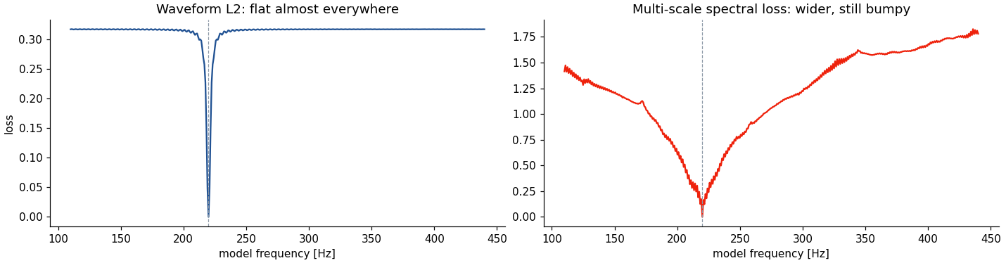
\[L_\text{MSS} = \sum_{n \in \{256, 1024, 4096\}} \frac{\big\| |S_n| - |\hat S_n| \big\|_1}{\| S_n \|_1} + \big\| \log(|S_n| + \epsilon) - \log(|\hat S_n| + \epsilon) \big\|_1\]

The loss slide follows the WS25 guest lecture by Gloria Dal Santo. MSS is what every fit in this lecture uses.

Failure case: a loss that cannot see a frequency

One decaying sine at 220 Hz, and a model sine whose frequency sweeps from 110 to 440 Hz.

• waveform L2: flat until the model is within a few Hz. No gradient points the way.
• spectral loss: a wider basin, still bumpy.

 

Practice

Do not learn what an analysis can measure. Pitch comes from a pitch tracker, delays from the room size; gradient descent refines decays, gains, filters and positions.

Structure: three fits

A guitar note: fit lecture 9’s string

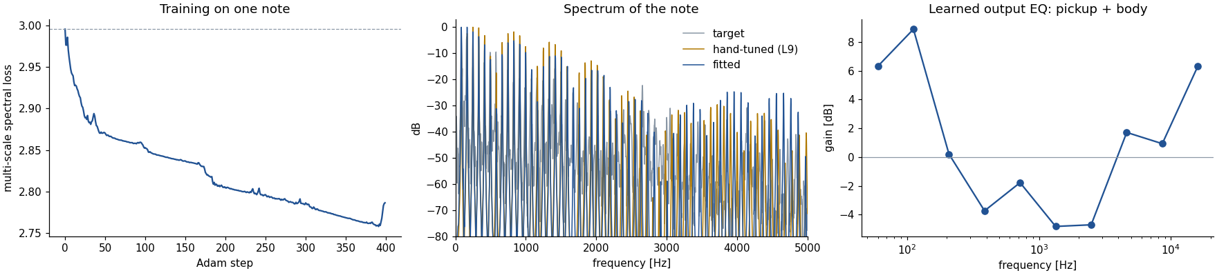
Parameter	By ear (L9)	Fitted
\(f_0\)	83 Hz, tracked	83 Hz (fixed)
stiffness \(B\)	\(5.0\cdot10^{-5}\)	\(6.4\cdot10^{-5}\)
\(\sigma_0\)	6.0	7.1
\(\sigma_2\)	\(1.0\cdot10^{-6}\)	\(5.6\cdot10^{-7}\)
pick, pickup	0.15, 0.03	0.15, 0.03
pick width	1.5 %	0.3 %

 

• trained on one note (the opening E2), 400 Adam steps
• learned: the physics and a 10-band output EQ for pickup and body
• the EQ took over the brightness; \(\sigma_2\) shrank to compensate
• the pick got harder: a narrower contact, more high modes

Did it learn the string, or the note?

Test on the 13 other notes of the riff, which training never saw (each at its own measured pitch):

Note	\(f_0\)	Loss, by ear	Loss, fitted
E3	165 Hz	2.86	2.70
D3	147 Hz	3.53	3.26
G3	196 Hz	3.62	3.54
A2	110 Hz	2.84	2.66
B2	123 Hz	3.63	3.44

… and better on all 13, by 1–14 % (6 % on average).

 

The whole riff, one fitted string:

target
by ear (L9)
fitted

Why it generalizes

The structure is shared by every note: one string, one body. What was fitted on one note is a property of the instrument, not of the recording.

A piano: when the loss and the goal disagree

The DDSP piano notebook (DDSP_Piano.py): one Pianoteq note, a 3-delay FDN whose delays are the three strings of a unison and whose matrix is the bridge; about 50 parameters.

	Training loss	Mean \(T_{60}\) error per partial
200 Adam steps	baseline	25 %
500 Adam steps	10 % lower	31 %

 

Failure case: overfitting the objective

The loss kept improving, the model got worse at what we care about (the decay of each partial). Past a point the extra steps fit fine structure no decay estimator measures.

Keep an exam

A measure the optimizer never sees: held-out notes, a physical quantity, a listening test.

An amplifier: sounds right, is wrong

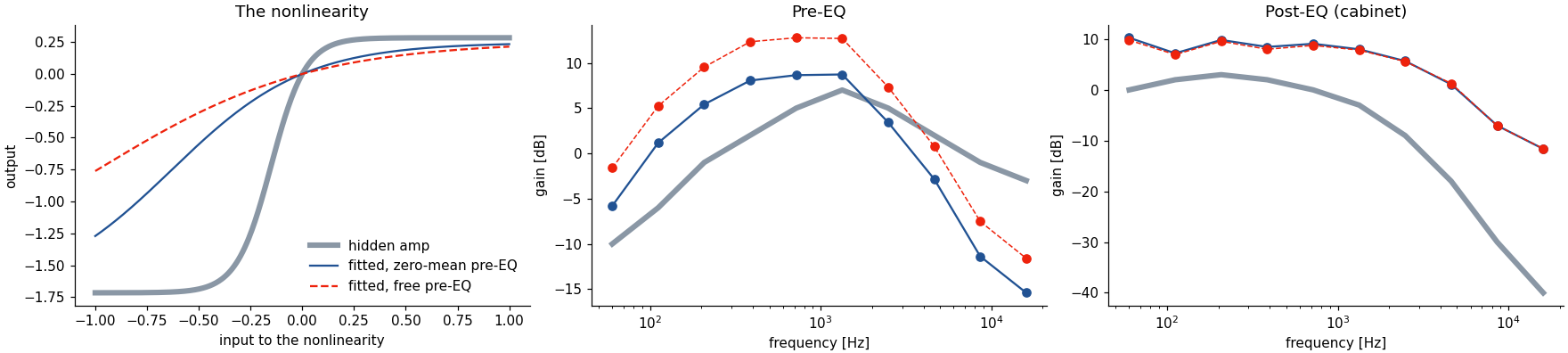
Grey box: pre-EQ → \(\tanh(g(u+b))\) → cabinet EQ, 22 parameters, fitted to a hidden amp on one guitar recording. On a different recording: loss 1.78 → 0.27.

 

But: drive \(g\) = 1.6 instead of 6, bias 0.63 instead of 0.15

At the true parameters the loss is exactly 0; the fit found a valley of nearly equivalent amps with a softer curve and more EQ. Sound matched, parameters not identified.

Even constraining the pre-EQ to zero mean (removing the exact level/drive trade-off) and starting at drive 3 or 10 ends at drive ≈ 2. White-box circuit models (Max’s WDFs) avoid this by fixing the component values; black boxes avoid it by not having parameters at all.

The parameters survive training

	Black box (network)	Grey box (DDSP)	White box (lectures 7–9)
Needs	lots of input–output data	a structure and some data	a structure and measurements
Knobs after training	only those it was trained with	all of the model’s: pluck position, \(T_{60}\), drive	all
Generalizes	within the training data	along the structure (other notes, other rooms)	wherever the physics holds
Parameters mean something	no	if they are identifiable	yes

Make it playable

After fitting the guitar string, which parameters would you now give to a player, and which would you freeze as “the instrument”?

A good answer: freeze the body EQ, stiffness and damping (the instrument); expose pluck position, pickup and excitation (the performance). The fit decides the instrument; the player decides the performance.

Match

Every lecture’s last step

Lecture	Structure	Matched by ear	Matched by gradient
7 · oscillators	saw + filter	cutoff envelope	amplitudes and filters (DDSP)
7, 9 · drums	808 voices, modal membrane	decay, snappy, strike position	inharmonic sines + noise + a learned transient (Shier et al. 2023)
8 · samples	the recording	nothing to match	the neural vocoder’s generator
9 · physical models	modal string	\(B\), \(\sigma\), positions	the same, plus a body EQ
10 · amps	EQ → nonlinearity → EQ	the drive knob	all 22, with a catch
11 · reverb	FDN	delays, \(T_{60}\)	absorption, EQ, matrix (next lecture)

Next lecture puts every method of the course into one room. Lecture 12 then removes the last hand-designed part: the structure itself. A diffusion model learns the representation and the generator from data.

Wrap-up

The four questions, for DDSP

	Black box	Grey box (DDSP)
Representation	network weights	the parameters of a DSP structure
Controls	the conditioning inputs	the structure’s own knobs
Built-in structure	none (or architecture only)	oscillators, filters, delays, physics
Fixed vs. learned	everything learned	structure fixed, numbers learned

Take away

Structure plus gradients

Write the DSP differentiably, choose a loss, let gradient descent do the match step. The structure makes the result generalize and keeps it playable.

 

The loss decides

What the loss cannot see, the fit cannot learn: frequencies from waveform losses, decays from spectrograms. Measure what you can, optimize the rest.

 

Keep an exam

A lower loss is not a better model, and a good-sounding fit need not have the true parameters. Test on held-out notes, rooms and quantities.

Further reading

• J. Engel, L. Hantrakul, C. Gu, A. Roberts, “DDSP: Differentiable digital signal processing,” ICLR 2020
• B. Hayes, J. Shier, G. Fazekas, A. McPherson, C. Saitis, “A review of differentiable digital signal processing for music and speech synthesis,” Frontiers in Signal Processing, 2024
• A. Wright, E.-P. Damskägg, V. Välimäki, “Real-time black-box modelling with recurrent neural networks,” DAFx 2019
• C. J. Steinmetz, N. J. Bryan, J. D. Reiss, “Style transfer of audio effects with differentiable signal processing,” J. Audio Eng. Soc., 2022
• S. Shan, L. Hantrakul, J. Chen, M. Avent, D. Trevelyan, “Differentiable wavetable synthesis,” ICASSP 2022
• F. Caspe, A. McPherson, M. Sandler, “DDX7: Differentiable FM synthesis of musical instrument sounds,” ISMIR 2022
• J. Shier, F. Caspe, A. Robertson, M. Sandler, C. Saitis, A. McPherson, “Differentiable modelling of percussive audio with transient and spectral synthesis,” Forum Acusticum 2023
• J. Shier, C. Saitis, A. Robertson, A. McPherson, “Real-time timbre remapping with differentiable DSP,” NIME 2024 (a drum played into a differentiable 808-style synth)
• G. Dal Santo, K. Prawda, S. J. Schlecht, V. Välimäki, “Differentiable feedback delay network for colorless reverberation,” DAFx 2023
• G. M. De Bortoli, G. Dal Santo, K. Prawda, T. Lokki, V. Välimäki, S. J. Schlecht, “Differentiable active acoustics: optimizing stability via gradient descent,” DAFx 2024

Fits in this deck: slides/make_ddsp_media.py (PyTorch; numbers in data/ddsp/fit_results.txt). Reverb match from the pyFDN tutorial (DAFx 2026); piano numbers from DDSP_Piano.py. Loss overview after the WS25 guest lecture by Gloria Dal Santo.