A History of Sound Synthesis
Lecture 1 · From tonewheels to diffusion models
160 years on one line
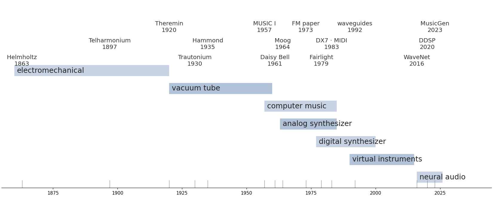
Each band is a technology; the methods ride on top of them. Additive synthesis was a dynamo in 1897, a spinning wheel in 1935, a computer program in 1957, and is a neural network’s output layer in 2020.
Helmholtz: timbre is a spectrum
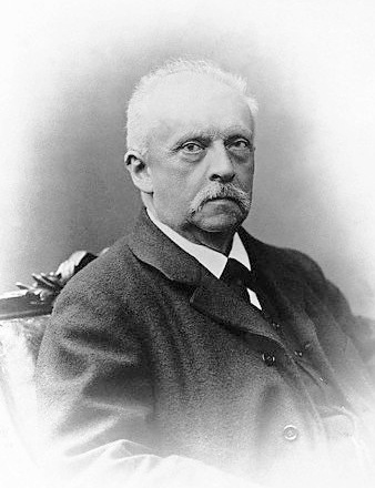 Hermann von Helmholtz (1821–1894)
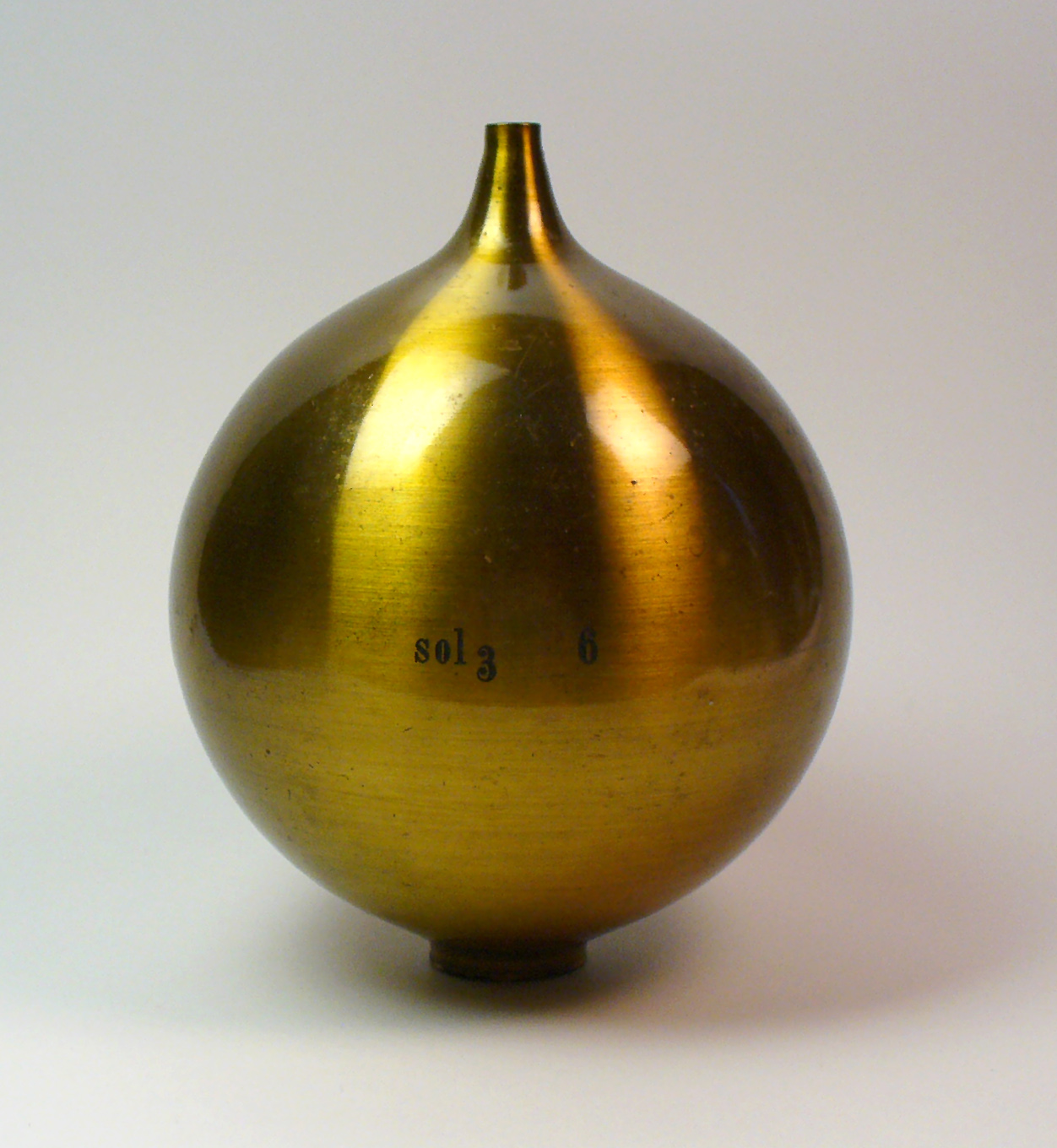 A brass Helmholtz resonator
H. v. Helmholtz, Die Lehre von den Tonempfindungen als physiologische Grundlage für die Theorie der Musik, 1863.
A tuned resonator held to the ear picks one partial out of a sound. With a set of them, Helmholtz measured the amplitude of every harmonic, and then rebuilt vowels with electrically driven tuning forks (120years): the first analysis-by-synthesis.
His claim, still the working assumption of every synthesizer: the ear hears the amplitudes of the harmonics, and mostly ignores their phases.
Build a tone, one harmonic at a time
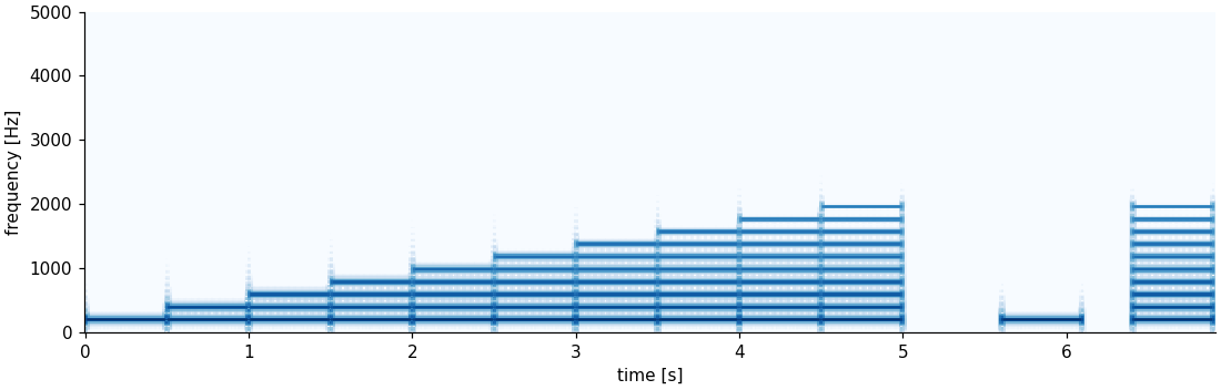
Ten half-second steps: harmonic \(k\) is added with amplitude \(1/k\); then the first and the last step again, side by side. The pitch never moves; only the timbre does, from a flute-like sine toward a sawtooth, \[x(t) = \sum_{k=1}^{K} \frac{1}{k}\,\sin(2\pi k f_0 t).\]
The Telharmonium: synthesis by dynamo
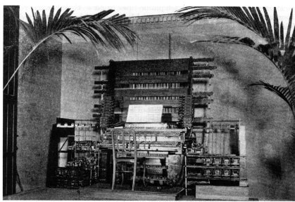 Thaddeus Cahill’s Telharmonium, patented 1897 · 120years
- One alternating-current dynamo per pitch, each a rotor whose shape sets the waveform
- Harmonics mixed from several dynamos: additive synthesis in iron and copper
- Mark II, 1906: about 200 tons, filled a floor of “Telharmonic Hall” in New York
- Music sold over telephone lines to hotels and restaurants, decades before radio
No recording of it survives. The first synthesizer was a streaming service, and it failed because its signals leaked into everyone else’s phone calls.
The theremin: pitch from a beat frequency
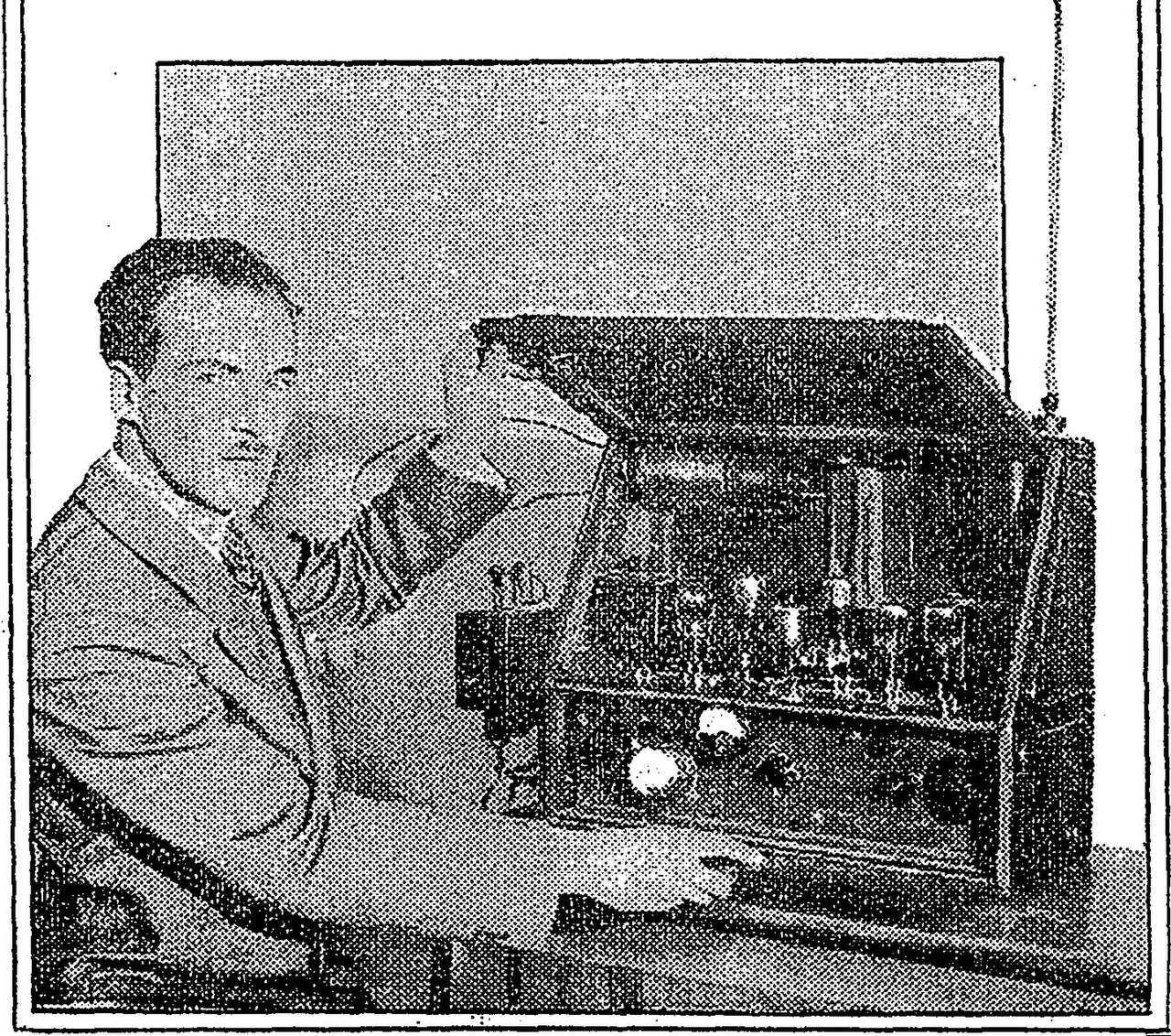 Leon Theremin and his instrument · 120years
Two radio-frequency oscillators, one fixed and one detuned by the capacitance of the player’s hand near the antenna. What you hear is their difference, \[f_\text{audio} = |f_\text{fixed} - f_\text{hand}|,\] so a change of a fraction of a percent at radio frequency sweeps the whole audible range. A second antenna sets the loudness. The player never touches the instrument.
Our clip is the principle: a sine with no discrete notes, continuous glides and a hand vibrato. The instrument’s difficulty is the same: there is nowhere to put your finger.
Trautonium and Ondes Martenot
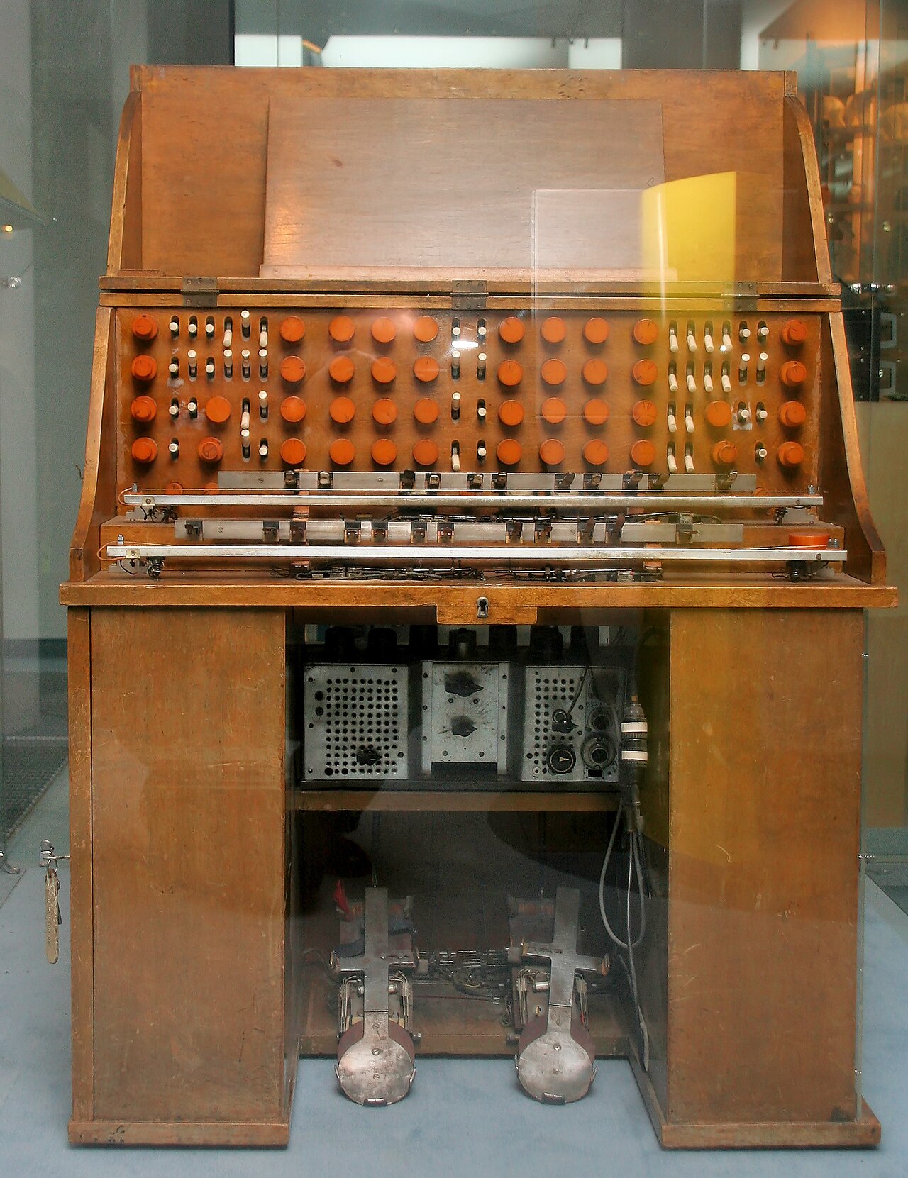 Mixtur-Trautonium · 120years
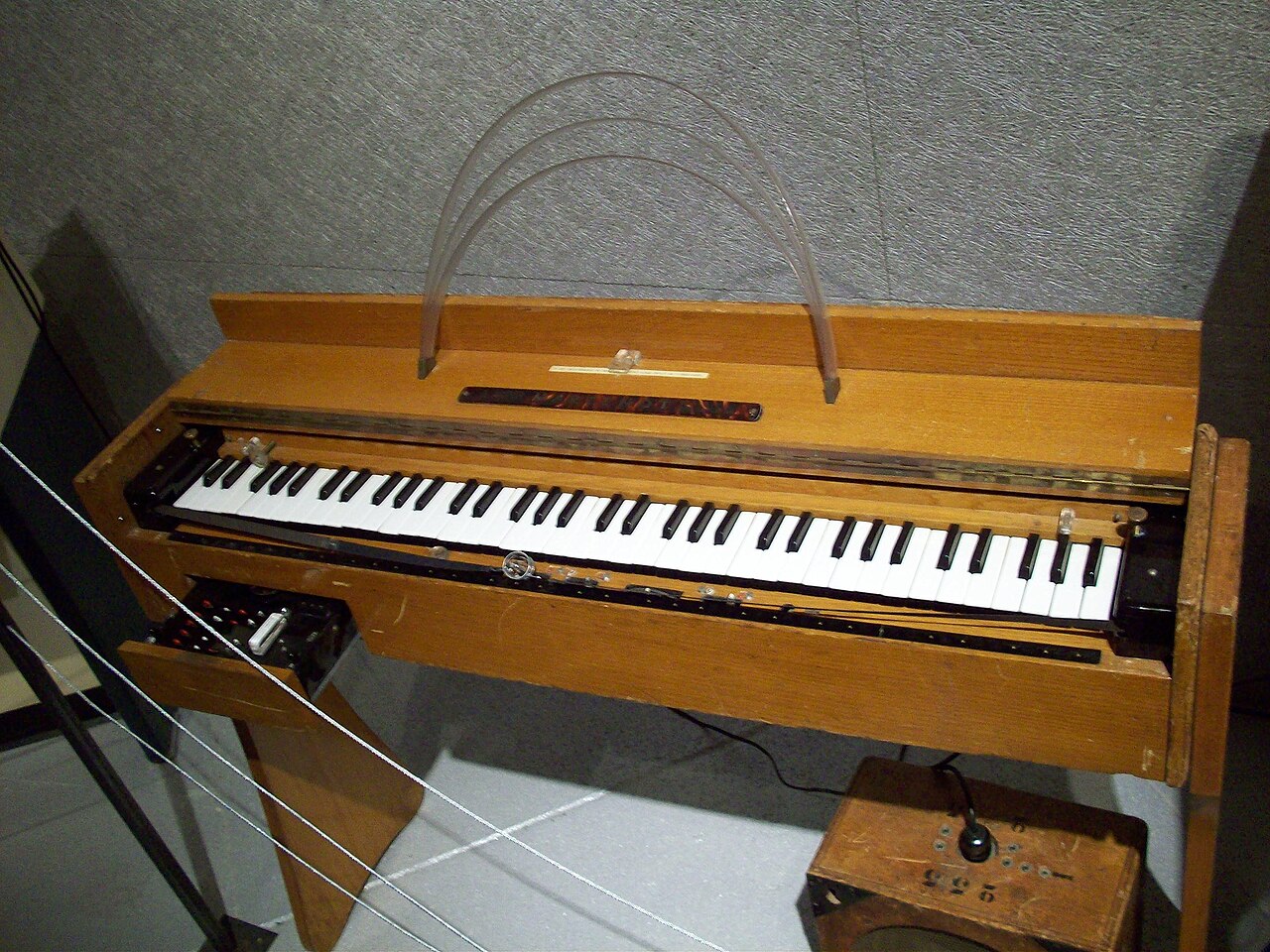 Ondes Martenot · 120years
Trautonium (Friedrich Trautwein, Berlin 1930). A wire pressed onto a metal rail sets the pitch; a sawtooth-like tube oscillator is shaped by resonant filters: subtractive synthesis, 34 years before Moog. Hindemith wrote a Konzertstück for it; Oskar Sala’s Mixtur-Trautonium made the bird sounds in Hitchcock’s The Birds (1963).
Ondes Martenot (Maurice Martenot, Paris 1928). A keyboard and a ring on a ribbon for glissandi, plus a pressure key for loudness. Messiaen’s Turangalîla; today Jonny Greenwood.
The Hammond organ: additive synthesis for the masses
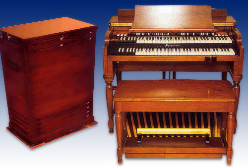 Hammond B3 with Leslie 122 · 120years
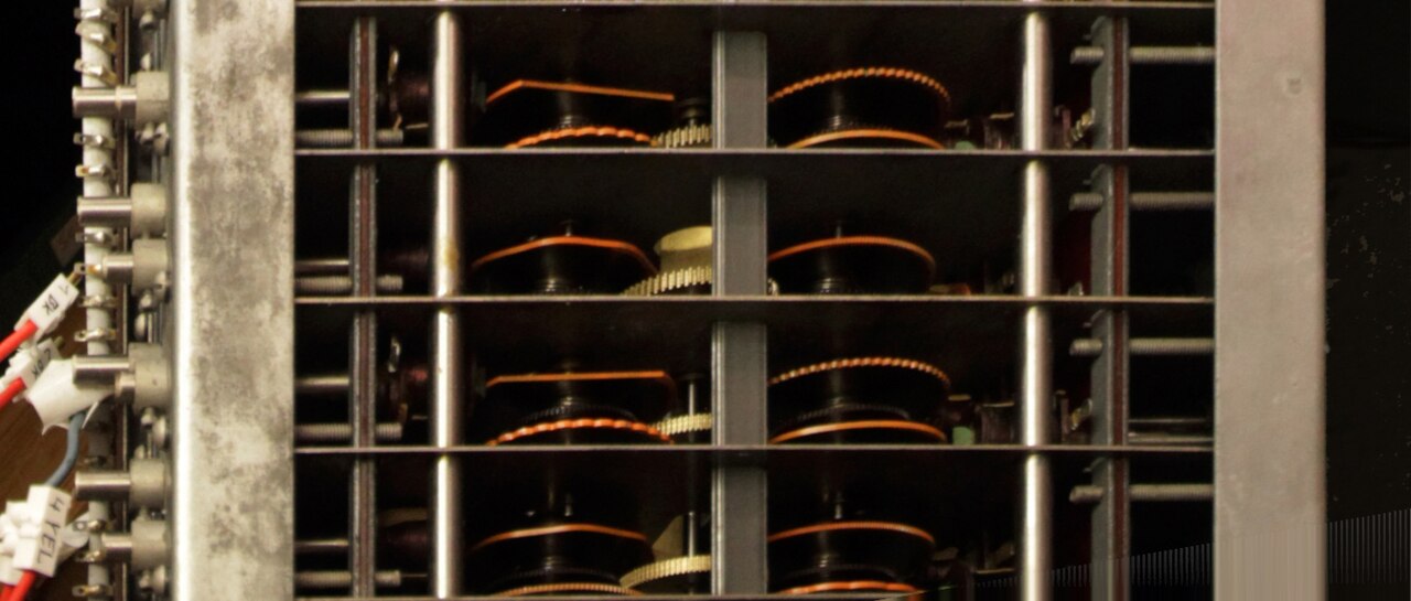 The tonewheel generator, from below
Laurens Hammond, 1935. One motor turns about ninety tonewheels; each is a toothed iron disk in front of a magnetic pickup and produces a near-sinusoid.
Nine drawbars mix the fundamental with eight other footages, each a volume from 0 to 8:
| Drawbar | 16′ | 5⅓′ | 8′ | 4′ | 2⅔′ | 2′ | 1⅗′ | 1⅓′ | 1′ |
|---|---|---|---|---|---|---|---|---|---|
| × \(f_0\) | ½ | 1½ | 1 | 2 | 3 | 4 | 5 | 6 | 8 |
That is Helmholtz’s table as a user interface. The gear ratios only approximate equal temperament, which is part of the sound.
Drawbars and the Leslie speaker
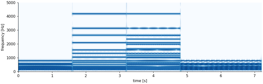
Registrations 888000000, 808808008, 888888888 (with key click), then 888000000 through a rotating Leslie horn: the rotation adds a Doppler shift (a periodically varying delay) and an amplitude modulation. Look for the wobble in the last chord’s partials.
Tape: sound as material
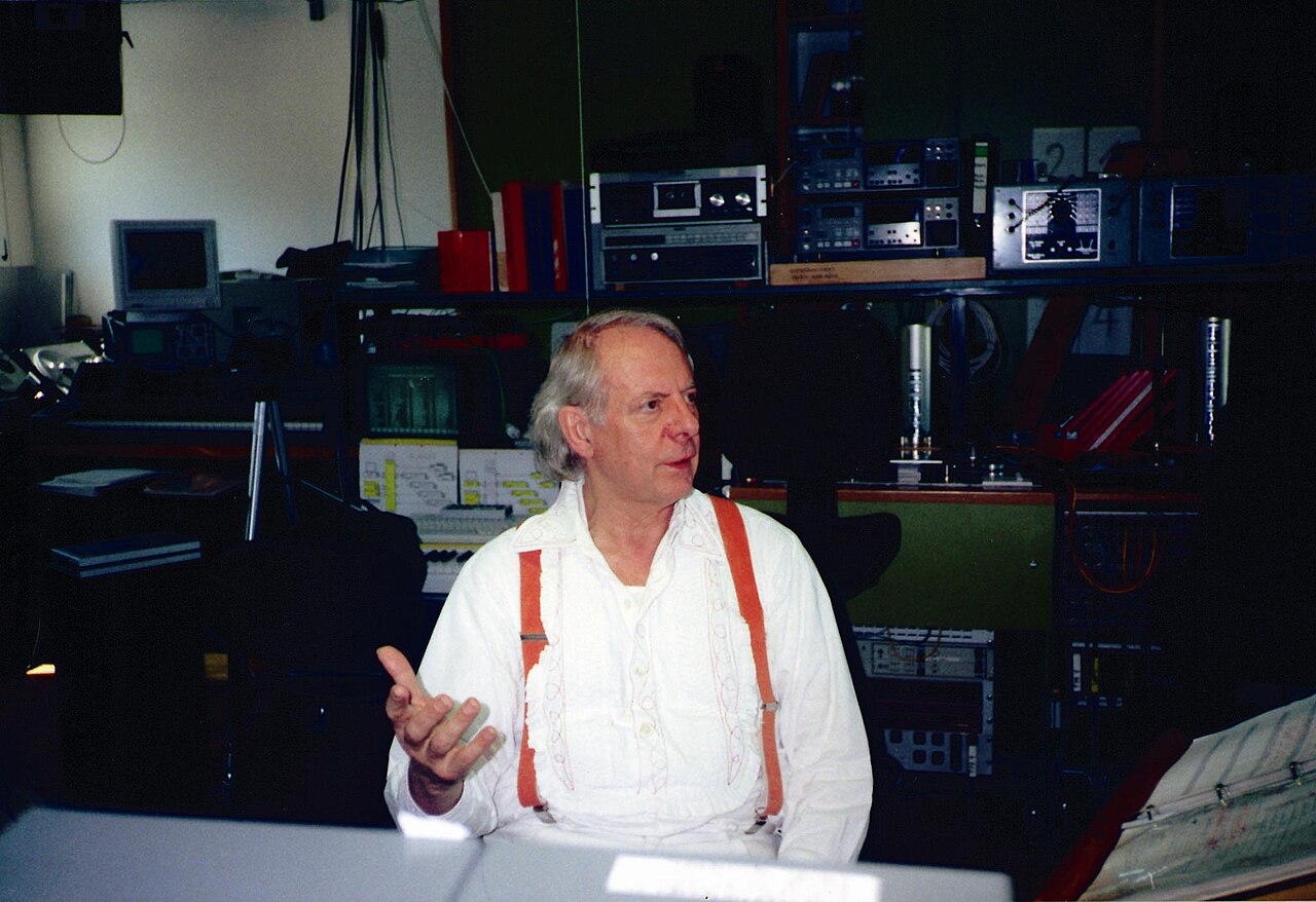 Karlheinz Stockhausen in his studio, 1996
- 1948, Paris: Pierre Schaeffer’s Étude aux chemins de fer, recorded trains cut and looped: musique concrète (120years)
- 1951, Cologne: the WDR Studio für elektronische Musik: sine generators and tape only (120years); Stockhausen’s Studie II (1954) is additive synthesis by scissors
- 1963, London: Delia Derbyshire realizes the Doctor Who theme at the BBC Radiophonic Workshop, every note a spliced piece of tape
Cut, splice, loop, change speed: these are sampling operations, forty years before samplers.
Max Mathews and MUSIC
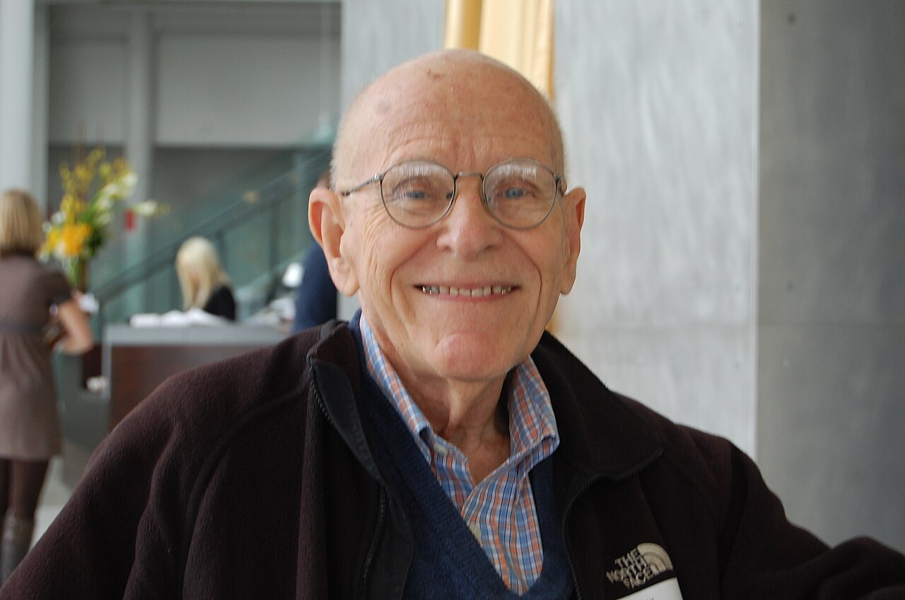 Max Mathews (1926–2011) · 120years: MUSIC N
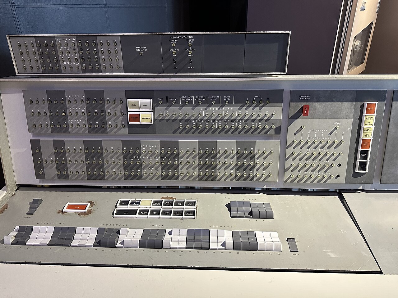 IBM 7094 console
1957, Bell Labs: MUSIC I on an IBM 704 computes a waveform sample by sample, writes it to tape, and a digital-to-analog converter plays it back. Seventeen seconds of music took hours.
MUSIC III (1960) introduced the unit generator: an oscillator, an envelope, a filter, patched into an instrument and driven by a score. Csound, Max, Pure Data, SuperCollider, every plugin graph, and PyTorch audio modules are that design.
M. V. Mathews, “The digital computer as a musical instrument,” Science 142, 1963.
Risset: synthesis as a microscope
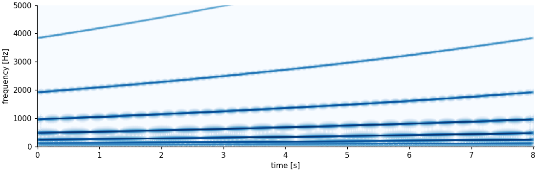
Jean-Claude Risset at Bell Labs, 1960s:
- Trumpet study (1965): its brightness grows with loudness; resynthesize the trumpet with that one rule and listeners cannot tell it from the recording
- Endless glissando: octave-spaced partials under a fixed bell-shaped spectral envelope. The clip rises forever and never arrives
Synthesis is also a test of understanding: a model of a sound is right when its resynthesis is indistinguishable from the original. The same criterion decides whether a neural model works.
And someone solved the wave equation
L. Hiller and P. Ruiz, “Synthesizing musical sounds by solving the wave equation for vibrating objects,” J. Audio Eng. Soc. 19, 1971.
Discretize the string in space and time and step it forward: \[y_{m}^{n+1} = 2y_m^n - y_m^{n-1} + \lambda^2\,(y_{m+1}^n - 2y_m^n + y_{m-1}^n)\] with Courant number \(\lambda = c\,\Delta t/\Delta x \le 1\).
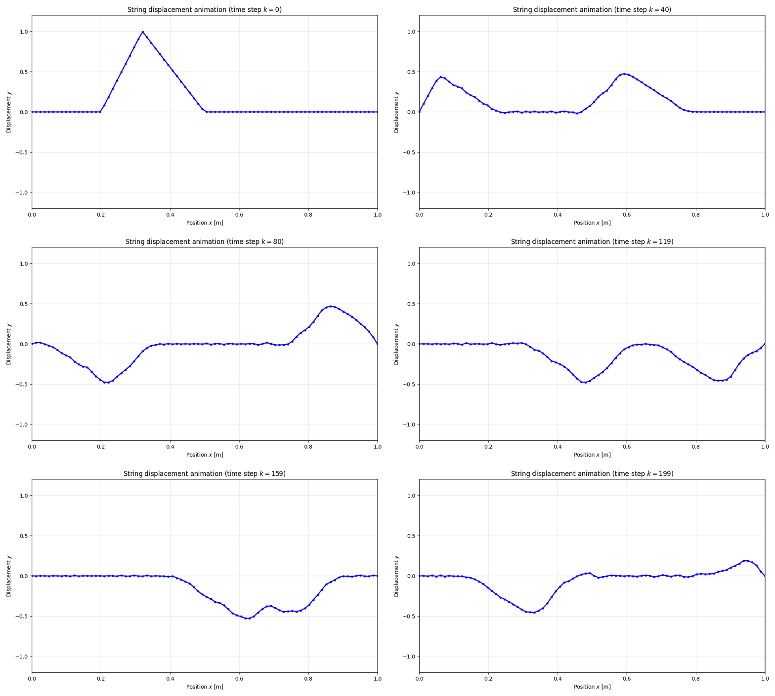
In 1971 this needed minutes of mainframe time per second of sound. Today it runs in real time, and we build it in this course. ▶ FDTD notebook
Voltage control
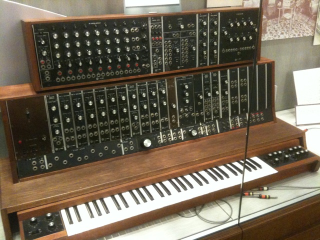
1963 Don Buchla (San Francisco Tape Music Center) and 1964 Robert Moog (New York) build modular synthesizers from transistor circuits. Every parameter is a control voltage, so any module can drive any other.
Moog’s key choice: an exponential converter, one volt per octave, \[f = f_0 \cdot 2^{V/1\,\mathrm{V}}.\] Pitch perception is logarithmic, so a linear keyboard voltage gives equal-tempered steps, and adding voltages transposes. Buchla’s early designs were linear.
R. A. Moog, “Voltage-controlled electronic music modules,” J. Audio Eng. Soc. 13, 1965.
The Moog ladder filter
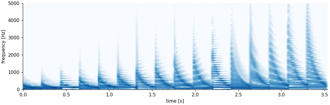
Four identical one-pole low-passes in series, with the output fed back to the input: \[H(s) = \frac{1}{(1 + s/\omega_c)^4 + 4k}.\] Near \(k = 1\) it resonates, near the cutoff, and then self-oscillates.
In the clip, each note opens the filter with an envelope, and the envelope depth grows over the phrase: watch the harmonics fan out upward. The \(\tanh\) in each stage is the transistor saturation that makes it sound like the circuit.
From the studio to the stage
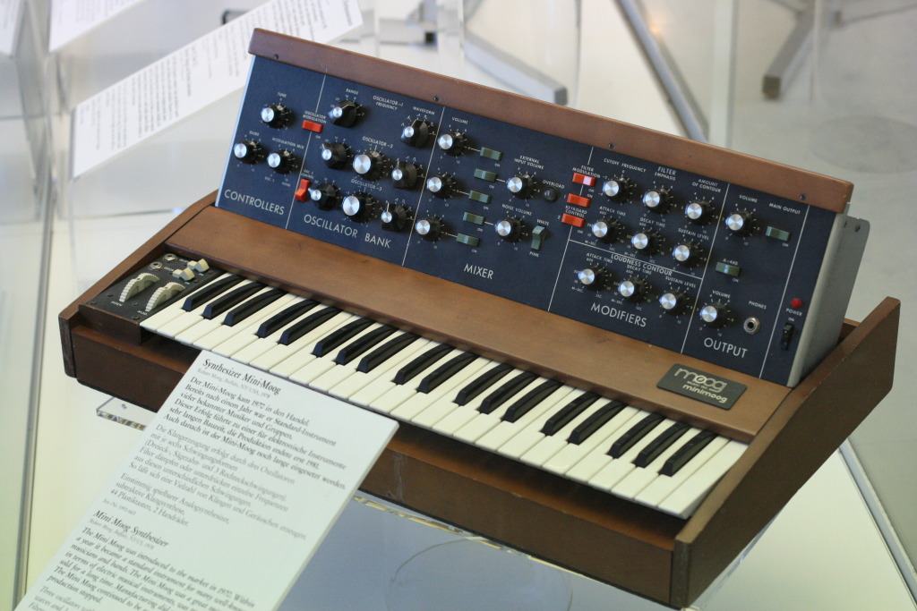 Minimoog, Deutsches Museum, München
| Year | |
|---|---|
| 1970 | Minimoog: the modular hard-wired into a portable box, about 12 000 sold |
| 1974 | Digitally scanned keyboards: polyphony |
| 1978 | Prophet-5: five voices, a microprocessor stores every knob position as a patch |
Bob Moog explains synthesis
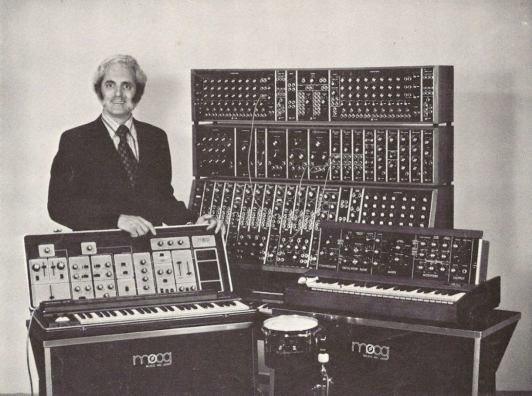 Robert Moog (1934–2005) with a modular system
The oscillator makes a waveform, the filter shapes its spectrum, the envelope shapes it in time: the whole of subtractive synthesis in under two minutes.
Chowning: frequency modulation
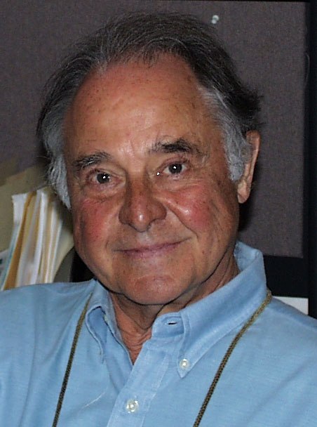 John Chowning
J. M. Chowning, “The synthesis of complex audio spectra by means of frequency modulation,” J. Audio Eng. Soc. 21, 1973.
Stanford, 1967: a vibrato made fast enough stops being heard as vibrato and becomes timbre: \[x(t) = A(t)\,\sin\!\big(2\pi f_c t + I(t)\,\sin(2\pi f_m t)\big) = A(t)\sum_{n=-\infty}^{\infty} J_n(I)\,\sin\!\big(2\pi(f_c + n f_m)t\big).\]
Two oscillators give a whole spectrum of sidebands at \(f_c \pm n f_m\), with weights set by the Bessel functions \(J_n\) of the modulation index \(I\). Let \(I\) follow an envelope and the brightness evolves like a real instrument’s, at the cost of one multiply-add per sample.
Three FM sounds
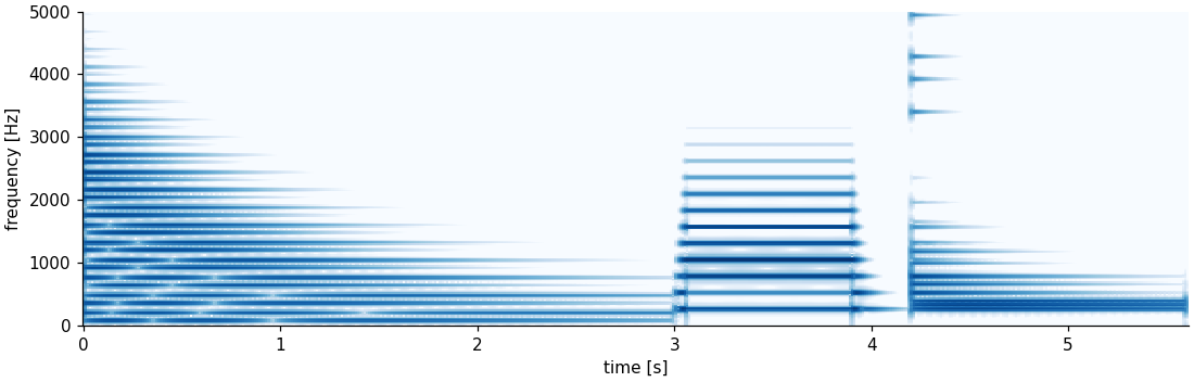
Bell: \(f_m/f_c = 1.4\), an inharmonic ratio, index decaying from 10. Brass: \(f_m = f_c\), index following the loudness envelope (Risset’s trumpet rule). E-piano: a 1:1 pair plus a high 14:1 “tine” pair with a short index decay, the recipe of the DX7’s most famous patch.
The Yamaha DX7
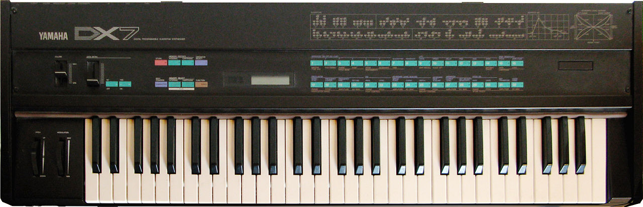 Yamaha DX7, 1983
- Six sine operators, 32 algorithms (which operator modulates which), 16 voices
- Stanford licensed the patent to Yamaha; it became one of the university’s most lucrative
- One of the best-selling synthesizers ever made; the sound of 1980s pop
The factory E.PIANO 1 patch
Chowning on the discovery (Stanford Historical Society)
The Mellotron: a tape per key
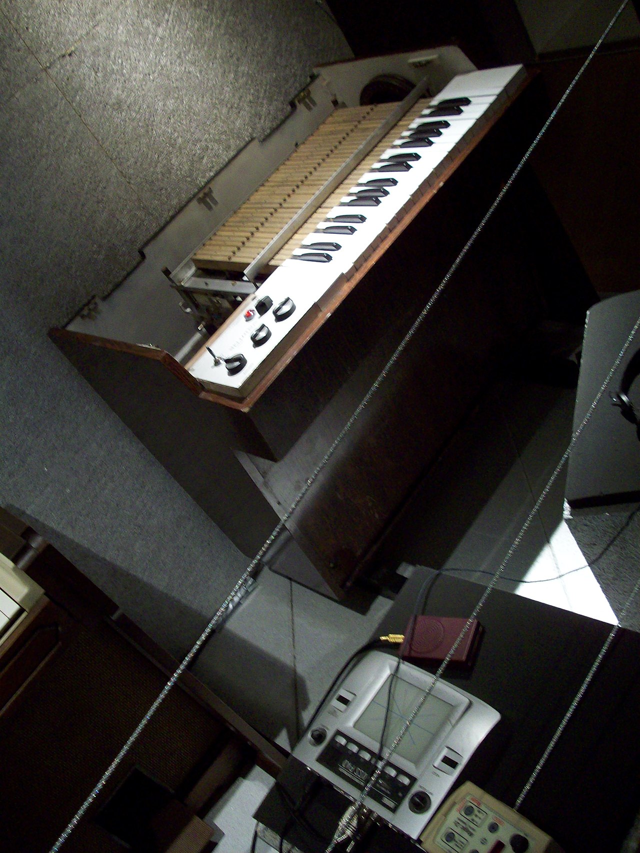 Mellotron · 120years
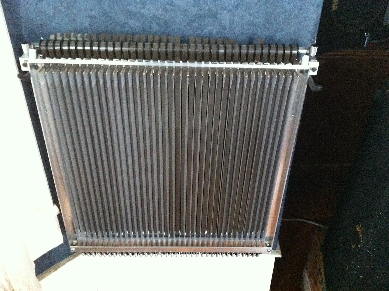 M400 tape frame: one strip per key
1963: each key presses an 8-second strip of tape against a turning capstan; releasing it lets a spring pull the tape back. No loops: hold a note longer than eight seconds and it stops.
Real flutes, choirs and strings, recorded once and replayed: sampling with analog storage. The flute that opens Strawberry Fields Forever (1967) is a Mellotron.
Digital sampling
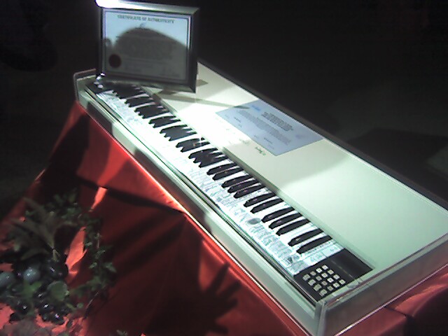 Fairlight CMI, 1979 · 120years
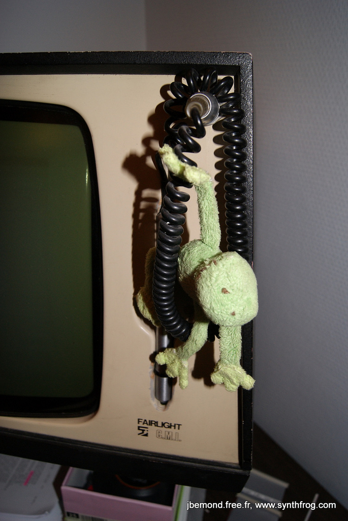 Its light pen: draw a waveform on screen
- 1979, Fairlight CMI (Sydney): digital recording, pitch-shifting and looping; Peter Gabriel, Kate Bush, and much of the 1980s
- 1981, E-mu Emulator makes it affordable
- 1984, Kurzweil K250: multi-sampling (a recording every few keys), convincing acoustic piano
The problem sampling creates: a recording is one performance. Transposing it changes its duration and formants; looping it needs a seamless loop point; it cannot respond to how you play.
Wavetables: sampling one period
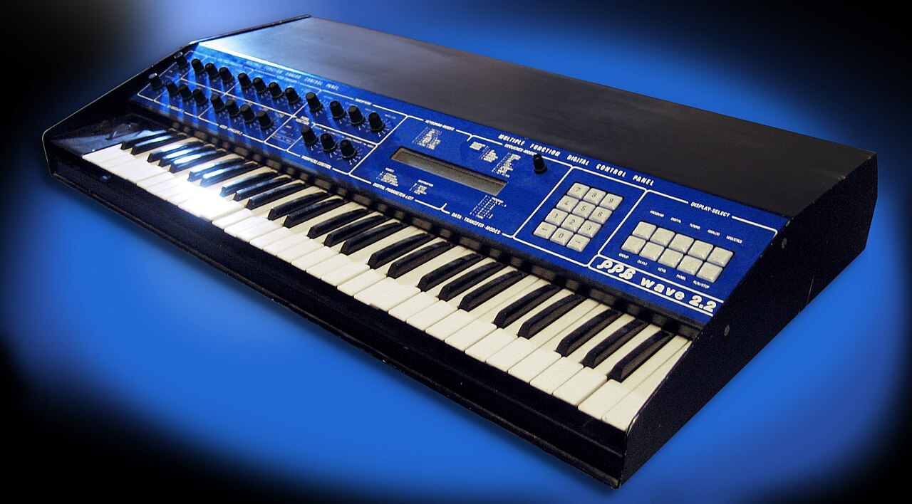 PPG Wave 2.2, 1982
Wolfgang Palm (Hamburg) stored 64 single-cycle waveforms per table. The oscillator plays one cycle and moves through the table while the note holds.
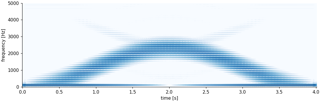
Our table morphs from a sine to a pulse with a moving formant; the scan goes up and back over four seconds. Memory in 1982 was the constraint, and one period is the smallest sample there is.
Karplus–Strong: a string in five lines
K. Karplus and A. Strong, “Digital synthesis of plucked-string and drum timbres,” Computer Music J. 7(2), 1983.
Fill a delay line of length \(N = f_s/f_0\) with noise, and feed it back through a two-point average: \[y[n] = x[n] + \tfrac{g}{2}\big(y[n-N] + y[n-N-1]\big).\] The loop keeps only the harmonics of \(f_0\); the average damps high ones faster, as a real string’s losses do.
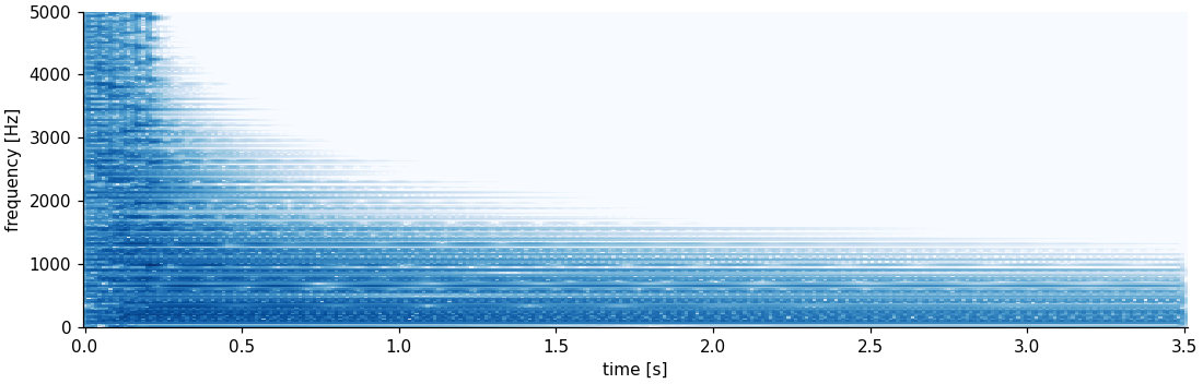
It was found as a wavetable trick, and recognized afterwards as a physical model: the delay is the travel time along the string and back.
Digital waveguides and modal synthesis
J. O. Smith III, “Physical modeling using digital waveguides,” Computer Music J. 16(4), 1992.
The d’Alembert solution: a string is two traveling waves, so simulate it with two delay lines and put all losses and dispersion into a few filters at the ends. Strings, bores, horns and vocal tracts, at the cost of a few operations per sample. 1994, Yamaha VL1: the first commercial physical-modeling synthesizer.
Or describe the object by its modes: a struck bar or bell is a sum of decaying sinusoids at inharmonic ratios (Adrien 1991; IRCAM’s Modalys).
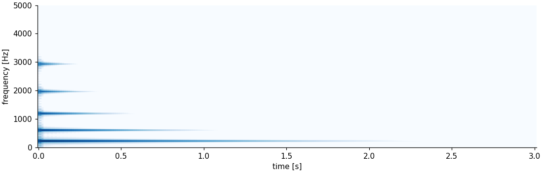
Which method made this?
Quiz
Three spectrograms from today. Name the synthesis method of each, and the feature that gives it away.
1
2
3
Answer
1 Karplus–Strong: exactly harmonic partials, the high ones dying first. 2 Wavetable: a fixed pitch whose spectral peak travels and returns. 3 Subtractive: a harmonic-rich source, filter envelopes fanning upward on every note.


.jpg)


_@_Stearns_Collection_(Stearns_2035),_University_of_Michigan.jpg)
.jpg)

_at_her_Theremin.jpg)
.jpg)


_Tongenerator_-_bottom_side,_closeup.jpg)
