Oscillators and Spectra

Lecture 7 · Additive, subtractive, FM, and waveshaping

Prof. Dr.-Ing. Sebastian J. Schlecht · Dr.-Ing. Maximilian Schäfer

Where we are

One question, asked of every method

Block	Representation	Generator
Filters and effects	LTI and time-varying systems	hand-designed
Classical synthesis	samples, partials, modes, physical state	hand-designed
DDSP	the same structured models	parameters learned
Reverberation	a recursive dynamical system	hand-designed, fittable
Diffusion	a learned representation	learned

 

The four questions

1. How is the sound represented?
2. What are the controllable parameters?
3. What structure is built in?
4. What is fixed by design, and what is learned?

The synthesis block in three lectures, from the waveform to the mechanism: today oscillators and spectra, then samples and grains, then physical models.

Listen

One riff, five instruments

the target: a real guitar
sine waves
sawtooth waves
sum of partials (additive)
filtered sawtooth (subtractive)

 

Listen first

Which one is closest to the guitar? What changes over the first 100 ms of a real pluck that the sine and the sawtooth do not do?

Same notes, same timing, transcribed from the recording. Only the way each note is written down differs.

Expected answers: the saw is too bright and too static; the pluck gets darker as it decays (high partials die first). The subtractive version gets that by moving a filter, the additive one by giving each partial its own decay. That is the whole lecture in one listening test.

Three ways to write down a tone

Representation	What is stored	What you control
one period (wavetable)	\(N\) samples of a single cycle	pitch, which table
a list of partials (additive)	frequency, amplitude, phase of every partial	every partial, over time
a rich source and a filter (subtractive)	a waveform shape and a filter	cutoff, resonance, envelopes
a modulated oscillator (FM, waveshaping)	two frequencies and an index, or a curve	index, ratio, drive

Each row trades memory, computation, and number of knobs differently. None of them knows it is imitating a guitar.

Represent

A periodic tone is a Fourier series

\[y(t) = \sum_{\nu=1}^{\infty} a_\nu \cos(\nu \omega_0 t + \varphi_\nu)\]

• \(\omega_0\) sets the pitch
• the amplitudes \(a_\nu\) set the timbre (Helmholtz, lecture 1)
• the ear barely hears \(\varphi_\nu\) for steady tones

Build a tone one harmonic at a time:

 

Single-cycle wavetable

Store one period as \(N\) samples, and read it with a phase accumulator: \[\phi[n+1] = \big(\phi[n] + f_0/f_s\big) \bmod 1, \qquad y[n] = T\big(N\phi[n]\big)\] Any spectrum, one table look-up per sample.

The table is the Fourier series, evaluated in advance.

Wavetables today: scan through a stack of periods

In the PPG Wave (early 1980s) and in today’s Serum and Vital, a wavetable is a stack of single-cycle waves, and the sound comes from scanning through it while the note plays.

The table position is a single knob that moves the whole spectrum, a first example of a macro control.

 

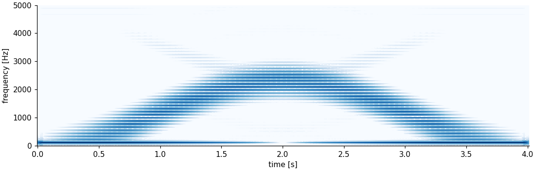
Scanning a 64-frame table up and back over four seconds.

Recorded-sample playback, looping and pitch shifting of whole notes are next lecture (samples and grains). Here the table is one period and only stands in for a spectrum.

Structure: additive

Additive synthesis: oscillators in parallel

 

• a linear system: exact, predictable control of every partial
• every partial can have its own envelope \(a_\nu(t)\) and its own frequency \(\omega_\nu(t)\)
• inharmonic partials cost nothing extra: bells, bars, stiff strings

Cost and control grow with the number of partials: a piano note has hundreds, each with its own envelope.

Risset analysed trumpet tones at Bell Labs in the 1960s this way: measure every partial’s envelope, resynthesise, and simplify until the ear notices. That is analysis-synthesis, and it comes back with the vocoder later today.

Additive pluck: where do the numbers come from?

An ideal string plucked at relative position \(p\):

\[a_\nu \propto \frac{\sin(\nu\pi p)}{\nu^2}, \qquad a_\nu(t) = a_\nu\, e^{-\sigma_\nu t}, \quad \sigma_\nu = \sigma_0 + \sigma_2\,\omega_\nu^2\]

• pluck position removes every \(1/p\)-th harmonic
• high partials decay faster: the tone darkens as it rings

 

Spectrum from physics

Five numbers (\(f_0, p, \sigma_0, \sigma_2\), level) instead of hundreds of envelopes. The formula is the solution of the wave equation, which lecture 9 derives: this is modal synthesis, before we have called it that.

Too dull: a real pickup, a pick attack and a guitar body are all missing.

Aliasing

Failure case: the naive sawtooth

The obvious oscillator: \(y[n] = 2\phi[n] - 1\).

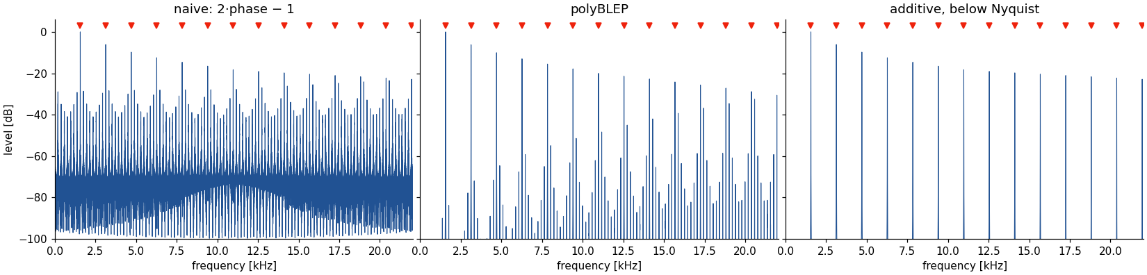
Its harmonics fall as \(1/\nu\) forever. Everything above \(f_s/2\) folds back to \(|f - k f_s|\): inharmonic tones that move the wrong way.

Saw sweep 100 Hz → 5 kHz:

naive
polyBLEP
additive, below Nyquist

 

Listen for

In the naive sweep: the whistling tones that fall while the pitch rises. Where do they come from?

A harmonic at \(\nu f_0 > f_s/2\) appears at \(f_s - \nu f_0\). As \(f_0\) rises, the alias falls.

The spectrum of an alias

G6 (1568 Hz) at 44.1 kHz: only 14 harmonics (red markers) fit below Nyquist. The naive saw fills the gaps with folded partials at −30 to −60 dB, easily audible.

Three cures

Additive

Sum only the harmonics below \(f_s/2\). Exact, but one oscillator per harmonic, and the count changes with pitch.

 

Band-limited tables

One wavetable per octave, each with the harmonics that fit. Cheap; switch or crossfade tables as the pitch moves.

 

Correct the jump

Aliasing comes from the discontinuity. Subtract a short polynomial step (polyBLEP) around each wrap: two samples of extra work.

\[y[n] = 2\phi - 1 - \mathrm{BLEP}(\phi), \qquad \mathrm{BLEP}(\phi) = \begin{cases} 2u - u^2 - 1, & u = \phi/\Delta < 1\\ u^2 + 2u + 1, & u = (\phi-1)/\Delta > -1\\ 0 & \text{otherwise}\end{cases}\]

with \(\Delta = f_0/f_s\), the phase step per sample.

Stilson & Smith (1996) did the band-limited impulse train (BLIT); Välimäki & Huovilainen (2007) popularised the polynomial version. Every virtual-analog synth uses a variant of this.

Structure: subtractive

Subtractive synthesis: a rich source, carved

Subtractive: carve away

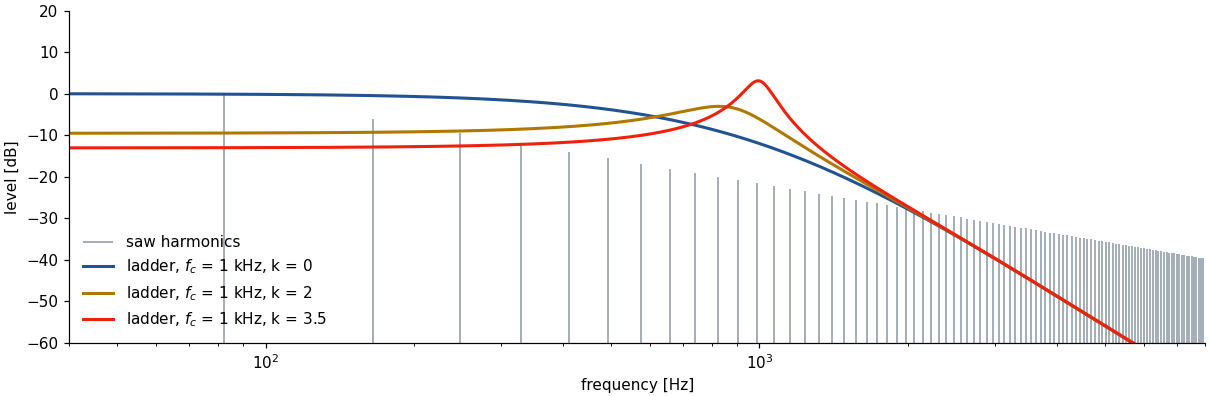
Start from a spectrally rich source \(x(t)\) and filter it: \[Y(j\omega) = H(j\omega)\,X(j\omega)\] Realized as serial filters, usually time-varying: exactly the filters of Max’s lectures.

 

The chain of every analog synthesizer since the Moog (lecture 1).

The resonant lowpass: four poles and feedback

Four one-pole lowpasses in series, the output fed back with gain \(k\):

\[H(z) = \frac{G(z)^4}{1 + k\,z^{-1}\,G(z)^4}\]

 

• \(k\) raises a peak at the cutoff
• \(k \to 4\): the filter oscillates by itself
• a \(\tanh\) at the input: the “analog” warmth

Cutoff sweep on a low saw:

\(k = 0\)		\(k = 3.3\)

Note the drop in passband gain as k grows, the characteristic Moog “bass loss” with resonance. Deriving the digital ladder properly (zero-delay feedback) is Max’s virtual-analog topic.

Subtractive pluck: move the filter, not the partials

\[f_c(t) = f_0\big(1.5 + 100\,v\,e^{-t/0.15\,\mathrm{s}}\big), \qquad a(t) = v\,e^{-t/0.6\,\mathrm{s}}\]

One envelope on the cutoff does what the additive model did with a decay per partial: the high partials die first.

target
subtractive

 

Additive vs. subtractive

Additive: many parameters, each with a meaning. Subtractive: few parameters, each moving many partials at once. The second is easier to play; the first is easier to fit.

Source and filter

Formant synthesis: source and filter

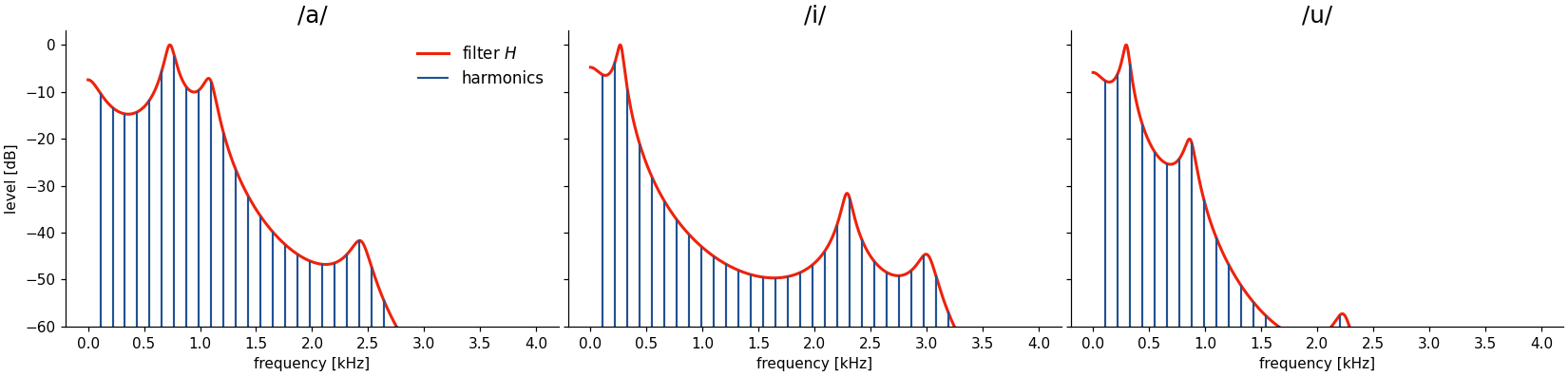
Real instruments and voices: a vibration excites a resonating body. Model both:

• source: oscillators (additive) plus noise
• body: filters with its resonances, the formants (subtractive)

 

Pulse train, then /a/, /i/, /u/: same source, three filters.

The harmonics stay where they are (multiples of 110 Hz); only the envelope moves. This is why pitch shifting a vowel sample sounds wrong: it shifts the red curve too. Next lecture.

The channel vocoder: analysis, then synthesis

Homer Dudley, Bell Labs, 1939: 10 band envelopes are enough to understand speech (120years: the Voder and Vocoder).

 

speech (modulator)
chord (carrier)
vocoder, 16 bands

Representation, then generator

The envelopes are a compact representation (a coarse spectrogram); the carrier and filters regenerate a waveform from it. Neural vocoders keep this split and learn the generator (lectures 8 and 10).

Modulation and nonlinearity

Many harmonics from two oscillators

Additive	FM
linear system	nonlinear system
oscillators in parallel	oscillators in series
harmonics ∝ oscillators	many harmonics from 2

 

	broadcasting	synthesis
\(\omega_m\)	audio	audio
\(\omega_c\)	≈ 100 MHz	audio
	\(\omega_c \gg \omega_m\)	\(\omega_c \approx \omega_m\)

J. Chowning, The synthesis of complex audio spectra by means of frequency modulation, J. Audio Eng. Soc., 1973.

Yamaha licensed it and sold the DX7 (1983): six operators, 32 algorithms.

FM in the time domain

\[x(t) = A \sin\!\big(\omega_c t + I \sin(\omega_m t)\big)\]

Instantaneous frequency: \[\omega(t) = \frac{d}{dt}\big(\omega_c t + I\sin\omega_m t\big) = \omega_c + I\omega_m\cos(\omega_m t)\]

• frequency deviation \(\Delta\omega = I\omega_m\)
• \(\omega_m \ll \omega_c\): vibrato
• \(\omega_m \approx \omega_c\): a new timbre

 

Index \(I\) swept from 0 to 8 at \(\omega_c = \omega_m\):

One knob, and the sound goes from a sine to a buzzy brass-like tone. That single parameter is why FM was so cheap: a DX7 voice is a handful of table look-ups and additions per sample.

The FM spectrum: Bessel functions

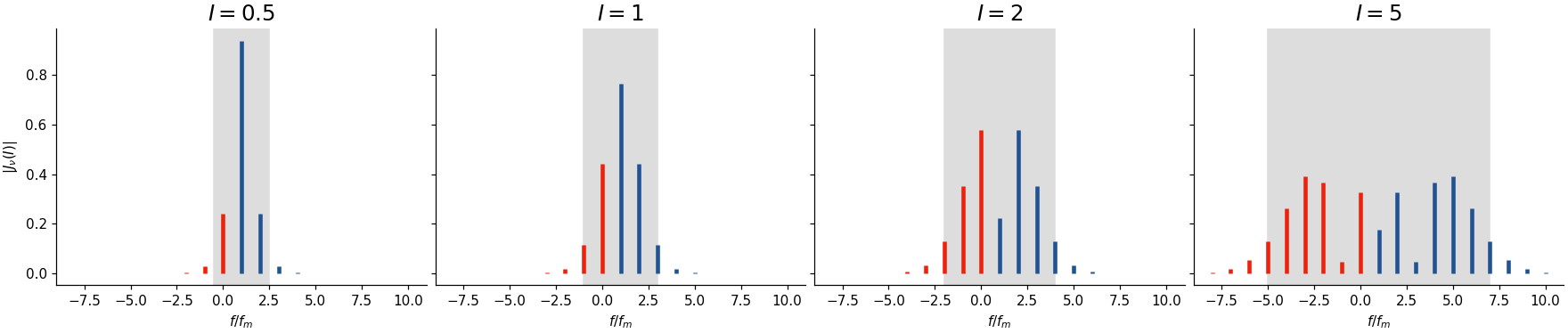
The modulating term \(e^{jI\sin\omega_m t}\) is periodic; its Fourier coefficients are Bessel functions of the first kind:

\[e^{jI\sin\omega_m t} = \sum_{\nu=-\infty}^{\infty} J_\nu(I)\, e^{j\nu\omega_m t} \quad\Rightarrow\quad x(t) = A\sum_{\nu=-\infty}^{\infty} J_\nu(I)\,\sin\big((\omega_c+\nu\omega_m)t\big)\]

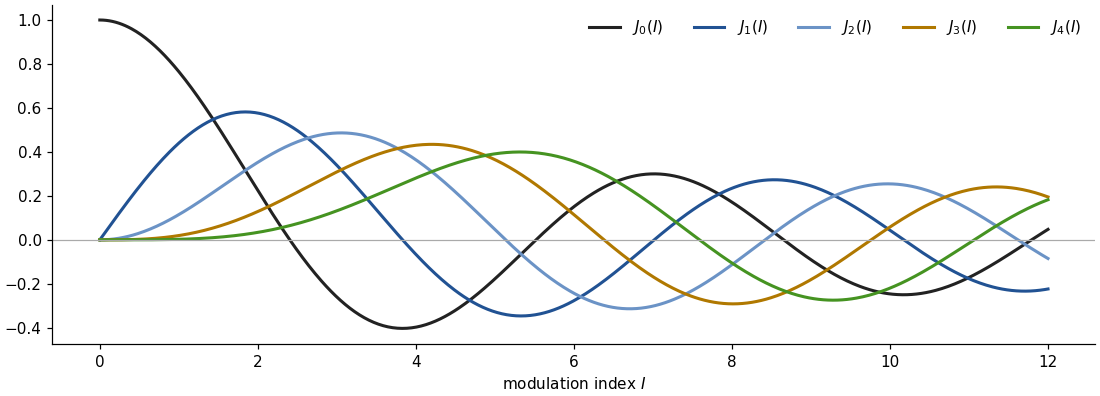
Small \(I\): \(J_0\) dominates, nearly a pure carrier. Larger \(I\): energy moves into the side bands \(J_1, J_2, \dots\), and at some \(I\) the carrier itself vanishes.

Reading an FM spectrum

• line spectrum, symmetric about \(\omega_c\), spacing \(\omega_m\)
• lines at negative frequency (red) fold back with a sign flip
• \(\omega_c : \omega_m\) rational → harmonic; irrational → inharmonic

 

Carson’s rule

About 99 % of the energy lies within \(\omega_B \approx 2(I+1)\,\omega_m\) (grey band). FM is not band-limited, so at high \(I\) it aliases: the failure case from before, again.

Sound design with FM

Couple the index to an envelope: \(x(t) = A(t)\sin\big(\omega_c t + I(t)\sin\omega_m t\big)\).

	Brass	Woodwind	Bell / percussion
Spectrum	all harmonics	odd harmonics	inharmonic
\(\omega_c : \omega_m\)	1 : 1	1 : 2	1 : 1.4
Index \(I(t)\)	follows \(A(t)\): louder = brighter	large at onset (chiff), then drops	decays with \(A(t)\)
Listen

Real patches use 4 to 7 operators in serial, parallel, and feedback arrangements (“algorithms”). Dexed is a free, open-source DX7 emulation for trying this.

Waveshaping: a curve instead of a filter

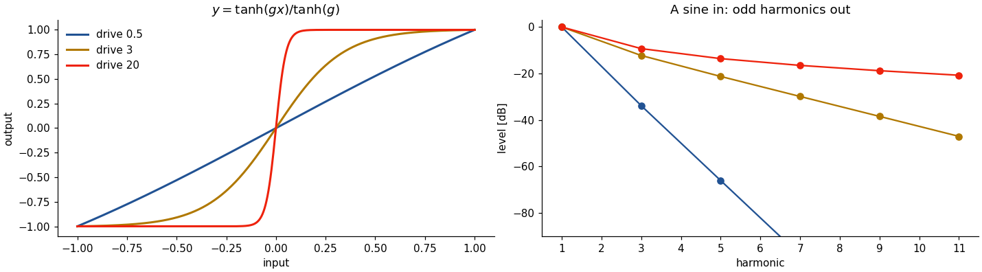
\[y[n] = f\big(x[n]\big)\]

• memoryless: no filter, no state
• an odd curve gives odd harmonics only

 

• drive is the index: louder in, brighter out
• Chebyshev polynomials \(T_\nu(\cos\theta) = \cos(\nu\theta)\) give exact control of each harmonic of a cosine input

Drive sweep on a sine:

Distortion and overdrive pedals from Max’s effects lectures are waveshapers with filters around them. In lecture 10 we fit exactly such a model to a guitar amplifier.

One family: put a nonlinearity somewhere

Method	Operation	What it adds	Knob
ring modulation	\(x(t)\cdot\sin\omega_m t\)	sum and difference frequencies	\(\omega_m\)
FM	\(\sin\big(\omega_c t + I\sin\omega_m t\big)\)	side bands at \(\omega_c \pm \nu\omega_m\)	\(I\), ratio
waveshaping	\(f\big(x(t)\big)\)	harmonics of the input	drive
nonlinear FDN (lecture 11)	\(f\) inside a feedback loop	harmonics, compounded every trip	\(\alpha\)

In every row, one index-like knob moves the sound from pure to rich. That makes them cheap and expressive, and it is also why none of them is easy to fit to a target.

Drums: oscillators and noise

An 808 is three recipes

	kick	snare	hi-hat (closed, open)
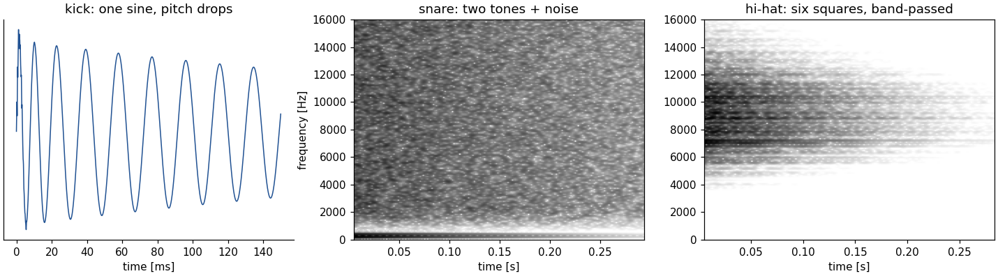
recipe	one sine, pitch falls from \(3f_0\) to \(f_0\) in ms	two damped sines (the head) + high-passed noise (the wires)	six squares at 205–800 Hz, band-passed to 7–11 kHz
listen

The Roland TR-808 (1980) does the kick and toms with pinged bridged-T resonant filters, which is why the pitch drop is a few milliseconds of the circuit settling. The six hat frequencies are the 808’s (Werner, Abel and Smith, ICMC 2014). Squares at those ratios give a dense inharmonic cluster, the band-pass keeps its top: it sounds like metal because nothing in it is harmonic.

Two knobs per drum

808 panel knob	what it moves
kick decay	\(\tau\) = 0.12 s
	\(\tau\) = 0.9 s
snare snappy	noise level 0
	noise level high

 

Put them on a 16-step sequencer:

Nothing here is a model of a drum. A drum is a short burst of energy into something that decays: a tone that drops, noise, an inharmonic cluster. The knobs are decay and mixture, not pitch and brightness. Lecture 9 models the membrane itself.

Control

Envelopes drive everything

ADSR

Attack, Decay, Sustain, Release: four corner points describe the amplitude envelope of almost every instrument sound.

The same four numbers, routed elsewhere:

• to the amplitude: loudness over time
• to the cutoff: brightness over time
• to the FM index or drive: richness over time

 

Real instruments

Brightness and loudness are coupled: a string plucked harder, a trumpet blown harder, a piano key struck harder are all louder and brighter.

Failure case: velocity as a volume knob

Velocity 0.3 → 0.6 → 1.0
amplitude only
amplitude and cutoff envelope depth

The first sounds like someone turning the volume; the second like someone playing harder. The difference is a mapping: one input (velocity) drives two parameters (level and brightness).

Make it playable

You may give a performer two knobs for the subtractive pluck and two for FM. Which?

Typical answers. Subtractive: brightness (envelope depth) and decay. FM: index (brightness) and ratio (harmonic vs. bell). The point: a good instrument hides most of its parameters behind a few perceptual controls, and the mapping is designed. Lecture 10 learns such mappings.

Match

How close did we get?

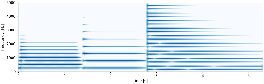
target
additive (string physics)
subtractive (tuned by ear)

What is still missing?

Listen to the first 50 ms of each note, and to the end of the long ones.

 

• the attack: pick noise, not a clean onset
• inharmonicity: a real string is stiff (lecture 9)
• the pickup and body filter
• interaction: a new note stops the old one on the same string

Two ways forward

Use the recording itself (lecture 8), or model the mechanism that makes all four (lecture 9). Either way, the parameters can be fitted instead of tuned by ear (lecture 10).

Wrap-up

The four questions, for oscillators

	Additive	Subtractive	FM / waveshaping
Representation	partials: \(a_\nu(t), \omega_\nu(t)\)	source shape + filter	two oscillators and an index, or a curve
Controls	every partial	cutoff, resonance, envelopes	index, ratio, drive
Built-in structure	linear, parallel	linear, serial	nonlinear
Fixed vs. learned	designed, or measured by analysis	designed	designed

Take away

Spectrum as representation

Additive writes the spectrum down partial by partial; subtractive carves it from a rich source; FM and waveshaping grow it with one index.

 

Aliasing

Discontinuities and nonlinearities make partials above Nyquist that fold back. Band-limit the source: additive, band-limited tables, or polyBLEP.

 

Control is a mapping

Envelopes and velocity couple loudness to brightness. Few perceptual knobs, many parameters behind them: the design problem of every instrument.

Further reading

• J. O. Smith III, Spectral Audio Signal Processing and Physical Audio Signal Processing, online books
• C. Roads, The Computer Music Tutorial, 2nd ed., MIT Press, 2023
• J. Chowning, “The synthesis of complex audio spectra by means of frequency modulation,” J. Audio Eng. Soc. 21(7), 1973
• M. Le Brun, “Digital waveshaping synthesis,” J. Audio Eng. Soc. 27(4), 1979
• T. Stilson, J. O. Smith, “Alias-free digital synthesis of classic analog waveforms,” ICMC 1996
• V. Välimäki, A. Huovilainen, “Antialiasing oscillators in subtractive synthesis,” IEEE Signal Processing Magazine 24(2), 2007
• A. Huovilainen, “Non-linear digital implementation of the Moog ladder filter,” DAFx 2004
• H. Dudley, “Remaking speech,” J. Acoust. Soc. Am. 11(2), 1939
• J.-C. Risset, M. V. Mathews, “Analysis of musical-instrument tones,” Physics Today 22(2), 1969
• K. J. Werner, J. S. Abel, J. O. Smith III, “The TR-808 cymbal: a physically-informed, circuit-bendable, digital model,” ICMC 2014

New examples in this deck: slides/make_oscillators_media.py. Drum examples: slides/make_drums_media.py. FM and formant examples: slides/make_synthesis_media.py. Guitar and speech recordings from the pyFDN audio set.