Lecture 9 · From the wave equation to modes, waveguides, and instruments
| Block | Representation | Generator |
|---|---|---|
| Filters and effects | LTI and time-varying systems | hand-designed |
| Classical synthesis | samples, partials, modes, physical state | hand-designed |
| DDSP | the same structured models | parameters learned |
| Reverberation | a recursive dynamical system | hand-designed, fittable |
| Diffusion | a learned representation | learned |
The four questions
Lecture 7 wrote down the spectrum, lecture 8 kept the recording. Neither could answer “what if I pluck it somewhere else?” Today: model the mechanism, and the answer is a parameter.
| The riff again | |
|---|---|
| target: the real guitar | |
| lecture 7: additive, ideal string | |
| today: modal string, struck by a pick near the bridge, damped, stopped by the next note |
One string, three questions a recording cannot answer:
| pluck in the middle | |
| pluck at the bridge | |
| strike with a hard hammer |
Listen first
What changed between the lecture-7 riff and today’s? Where do the attack and the short, muted notes come from?
Every method so far models the sound. A physical model simulates the object: a string, a tube, a membrane, including where it is struck and where it is heard.
The representation
Not samples of the output, but the state of the object: the displacement and velocity of every point of the string. The sound is what a pickup reads from that state.
The first milliseconds after a pluck: the deflection \(y(x,t)\) is a function of space and time.
\[\underbrace{\rho A\,\ddot y - T_s\,y''}_{\text{wave equation}} \;+\; \underbrace{EI\,y''''}_{\text{stiffness}} \;+\; \underbrace{d_1\,\dot y - d_3\,\dot y''}_{\text{damping}} \;=\; f_e(x,t)\]
Wave equation only: pulses travel unchanged at \(c_0 = \sqrt{T_s/\rho A}\)
+ stiffness: high frequencies travel faster, so the pulse spreads (dispersion)
+ damping: frequency-independent (\(d_1\)) and frequency-dependent (\(d_3\)) losses
Same string, stiffness increasing from left to right. Listen to the attack and the “twang”:
reference
none
more
more still
extreme
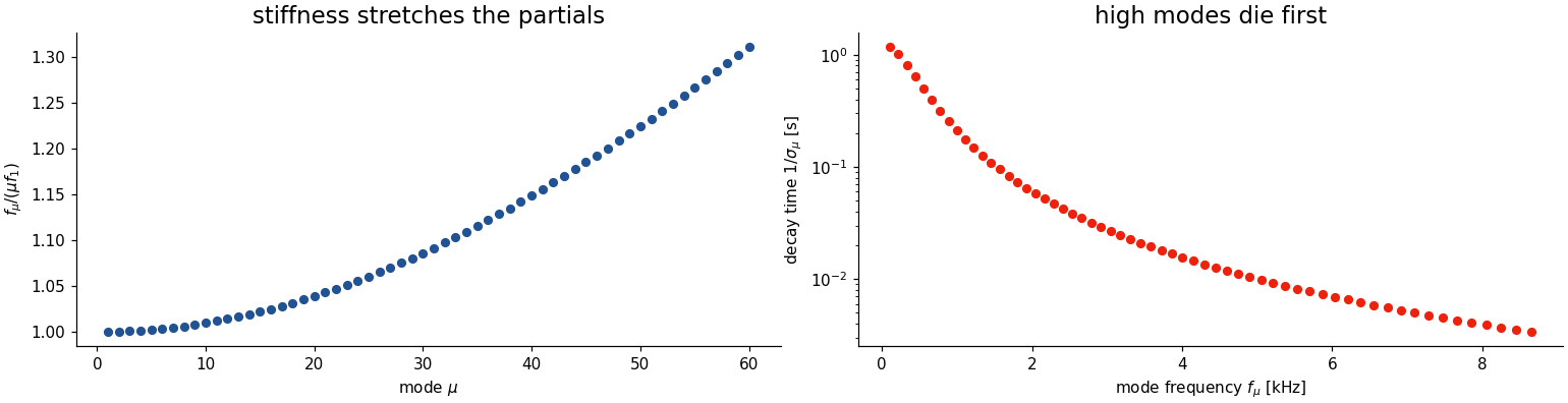
Stiffness stretches the partials: \(f_\mu \approx \mu f_1\sqrt{1 + B\mu^2}\). In a piano this inharmonicity is why octaves are tuned slightly wide, and why bass strings sound “metallic”.

Grid \(x_m = mh\), \(t_k = kT\); replace derivatives by central differences. For the wave equation \(\ddot y = c^2 y''\):
\[y_m^{k+1} = 2(1-\lambda^2)\,y_m^k + \lambda^2\big(y_{m+1}^k + y_{m-1}^k\big) - y_m^{k-1}\]
with the Courant number \(\lambda = cT/h\). Ends fixed: \(y_0^k = y_{N}^k = 0\).
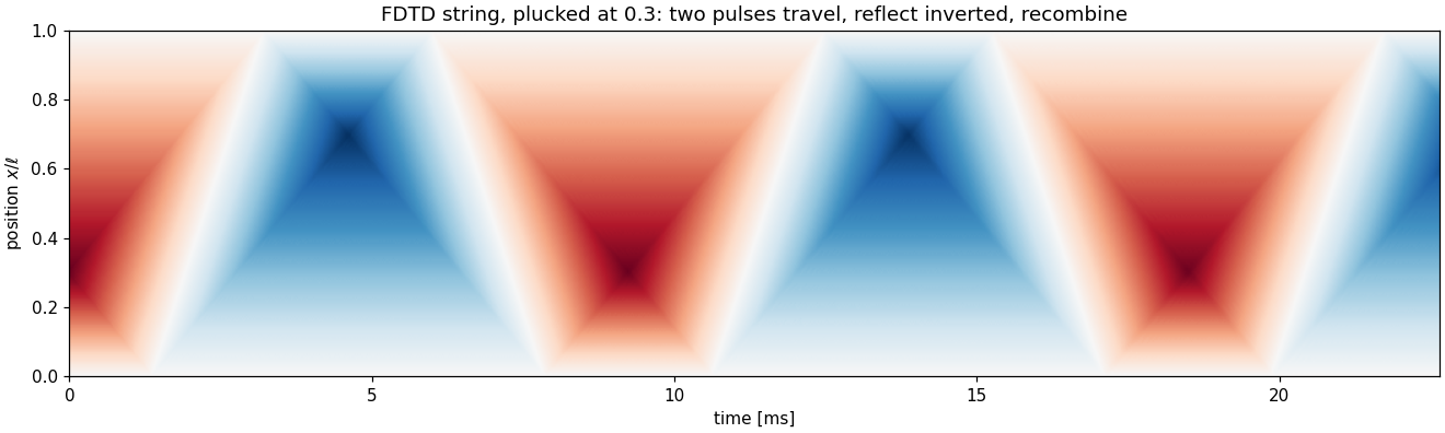
Add the two loss terms and pluck at 0.3 (200 grid intervals, ≈ 108 Hz):
The triangle splits into two pulses that travel, reflect inverted at the fixed ends, and recombine once per period.

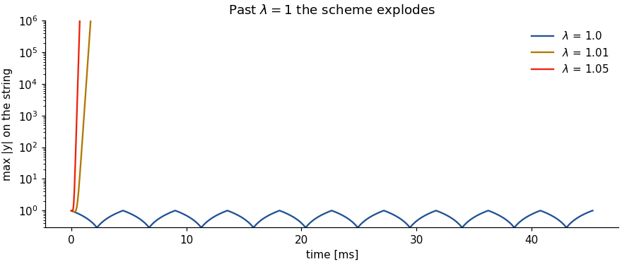
The explicit scheme is stable only for
\[\lambda = \frac{cT}{h} \le 1\]
A wave may not travel more than one grid step per time step. One percent over, and the string explodes within 2 ms.
Fixing \(f_s\) and the pitch fixes \(c/h\): a stiffer or higher string needs a coarser grid, and the grid sets how many modes you get.
Stack the grid into a vector \(\mathbf y^k\). The update is a matrix recursion with the discrete Laplacian \(\mathbf L = \operatorname{tridiag}(1, -2, 1)\):
\[\mathbf y^{k+1} = \big(2\mathbf I + \lambda^2 \mathbf L\big)\,\mathbf y^k - \mathbf y^{k-1} \qquad\Longleftrightarrow\qquad \underbrace{\begin{bmatrix}\mathbf y^{k+1}\\ \mathbf y^{k}\end{bmatrix}}_{\mathbf x[k+1]} = \underbrace{\begin{bmatrix} 2\mathbf I + \lambda^2 \mathbf L & -\mathbf I\\ \mathbf I & \mathbf 0\end{bmatrix}}_{\mathbf A} \underbrace{\begin{bmatrix}\mathbf y^{k}\\ \mathbf y^{k-1}\end{bmatrix}}_{\mathbf x[k]} + \mathbf b\, u[k]\]
Hold on to this form
Lecture 11’s reverb (the FDN) is \(\mathbf x[n+1] = \hat{\mathbf A}\mathbf x[n] + \hat{\mathbf b}\,x[n]\) too. A string and a reverb are the same kind of object: a large, sparse, recursive linear system.

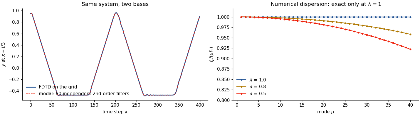
\(\mathbf L\) is symmetric: \(\mathbf L = \boldsymbol\Phi\boldsymbol\Lambda\boldsymbol\Phi^\top\), with discrete sines as eigenvectors. In modal coordinates \(\boldsymbol\eta = \boldsymbol\Phi^\top\mathbf y\) every mode runs on its own:
\[\eta_\mu^{k+1} = \big(2 + \lambda^2\beta_\mu\big)\,\eta_\mu^k - \eta_\mu^{k-1}\]
one second-order filter per mode, with poles on the unit circle at
\[\cos\Omega_\mu = 1 + \tfrac{\lambda^2}{2}\beta_\mu, \qquad \beta_\mu = -4\sin^2\!\frac{\pi\mu}{2N}\]
| Discrete (FDTD notebook) | Continuous (FTM) |
|---|---|
| central differences | the PDE itself |
| \(z\)-transform in time | Laplace transform in time |
| eigenvectors of \(\mathbf L\) | Sturm–Liouville transform in space |
| \(\beta_\mu\) of a finite grid | exact eigenvalues, all terms of the PDE |
| resonator per mode | resonator per mode |
Functional Transformation Method (FTM)
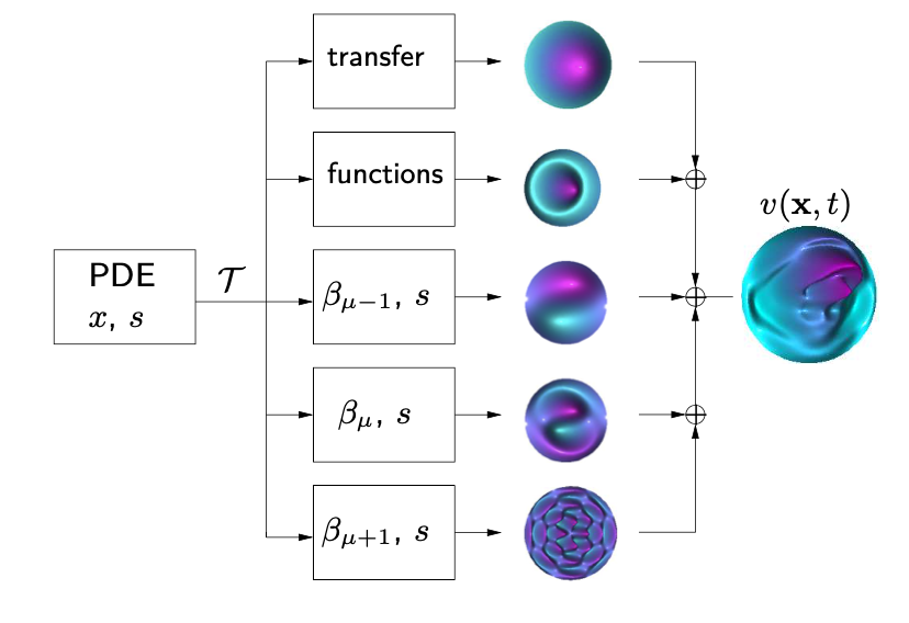
Transform the PDE with its boundary conditions into a set of independent second-order systems, then into discrete-time resonators. Exact modes, no spatial grid, no numerical dispersion. Stiffness and damping just move \(f_\mu\) and \(\sigma_\mu\).
L. Trautmann and R. Rabenstein, Digital Sound Synthesis by Physical Modeling Using the Functional Transformation Method, Kluwer, 2003.
full string motion
\(\mu = 1\)
\(\mu = 2\)
\(\mu = 3\)
\[y(x,t) = \sum_{\mu} \underbrace{\bar y_\mu(t)}_{\text{temporal: a damped sinusoid}} \;\cdot\; \underbrace{K_\mu(x)}_{\text{spatial: the mode shape}} \qquad \text{e.g. } K_\mu(x) = \sin\!\Big(\frac{\mu\pi x}{\ell}\Big)\]
Each temporal part \(\bar y_\mu(t) = e^{-\sigma_\mu t}\sin(2\pi f_\mu t)\) is the impulse response of a second-order IIR filter:
\[H_\mu(z) = \frac{b_\mu z^{-1}}{1 - 2 e^{-\sigma_\mu T}\cos(2\pi f_\mu T)\, z^{-1} + e^{-2\sigma_\mu T} z^{-2}}\]
The same structure as formant synthesis and as lecture 7’s additive pluck, but now every \(f_\mu\), every \(\sigma_\mu\) and every weight comes from the physics, and where you pluck and listen is a parameter.
The lossless wave equation \(\ddot y = c_0^2 y''\) has d’Alembert’s solution \[y(x,t) = y_l(x + c_0 t) + y_r(x - c_0 t)\] two shapes traveling left and right. Sample with \(x = mh\), \(t = kT\) and \(h/T = c_0\) (that is, \(\lambda = 1\)): \[y[m,k] = y_l[m+k] + y_r[m-k]\]
A traveling wave is a delay line. Two delay lines in opposite directions simulate the lossless string exactly, at the sample points, for one addition per output sample.
J. O. Smith III, Physical modeling using digital waveguides, Computer Music Journal, 1992.
The FDTD figure showed exactly this: two pulses, traveling and reflecting.
Insert filters \(H(z)\) into the lines:
| \(H(z)\) | models |
|---|---|
| \(1\) | lossless |
| \(0 < g < 1\) | frequency-independent loss (\(d_1\)) |
| low-pass | frequency-dependent loss (\(d_3\)) |
| all-pass | dispersion (stiffness) |
Boundaries reflect the waves: \(R(z) = -1\) for a rigid end, \(|R|<1\) for a lossy one, a filter for a bridge coupled to a soundboard.
Commute and combine
With one input and one output, all the delays merge into one delay line \(z^{-M}\) and all the filters into one loop filter. Add a fractional-delay filter to tune the pitch exactly.
Max built it from a feedback comb filter: a delay line, and a two-point average in the loop.
The waveguide explains why it works:
| Karplus–Strong | the string |
|---|---|
| delay line \(M\) | one round trip, \(2\ell / c_0\) |
| noise in the delay line | the initial displacement |
| averaging filter | \(d_3\): high partials lose more per trip |
| sign of the loop | the two inverting reflections |
From accident to model
Karplus and Strong (1983) found the sound by experiment. The waveguide (Smith 1992) shows it is the commuted, lossy string with the crudest possible loop filter. Replace the average by a designed low-pass and all-pass, and every parameter has a physical meaning.
The Karplus–Strong paper is titled “plucked-string and drum timbres”. One change in the loop: keep the averaged sample with probability \(b\), negate it otherwise, \[y[n] = \pm\tfrac12\big(y[n-M] + y[n-M-1]\big), \quad P(+) = b.\]
| \(b = 1\): the string | |
| \(b = \tfrac12\): a drum | |
| \(b = \tfrac12\), \(M\) three times longer |
Random signs destroy the periodicity, so there is no pitch, only a noise burst whose brightness and decay are set by the loop: \(M\) now acts as a decay-time knob, not a pitch. A cheap snare, and a hint that a drum is not a string with a different number.
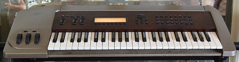
Yamaha VL1 (1994) · Daniel Hartwig, CC BY 2.0, cropped
Waveguides were the physical model of the 1990s: Yamaha VL1/VL7 (1994), Korg Prophecy (1995), sound cards from Creative.
oboe → bassoon
trumpet
tenor sax
Strong for 1D systems: strings, bores of wind instruments. 2D plates and membranes need waveguide meshes, which lose most of the efficiency.
Sound examples: J. O. Smith, CCRMA
| Waveguide | Modal / FTM | FDTD | |
|---|---|---|---|
| Represents | traveling waves | standing waves | the field on a grid |
| Best for | 1D, low loss: strings, bores | linear systems, any shape with known modes | nonlinear, coupled, complex geometry |
| Cost | lowest: a few delays and filters | one resonator per mode | every grid point, every sample |
| Weak at | 2D/3D, strong dispersion | nonlinearity (e.g. tension modulation) | numerical dispersion, stability limits |
Rule of thumb
Waveguides dominated when computers were slow. Now that they are fast, modal and FDTD methods win whenever the physics matters more than the budget. In every case: understand the physics of the instrument first.

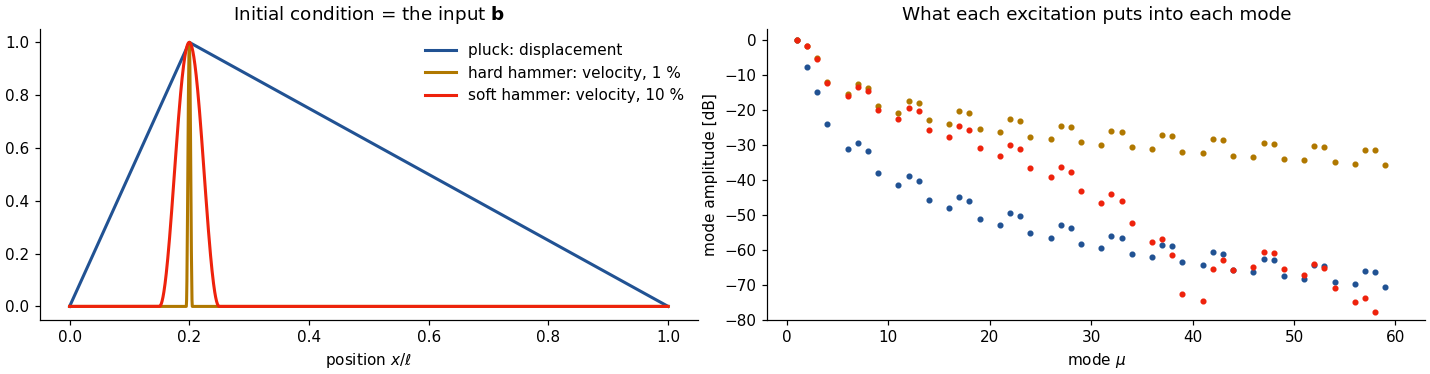
In state space the excitation is \(\mathbf b\) (or the initial state). Project it onto the modes: each excitation writes a different spectrum into the string.
| Same string, same position | |
|---|---|
| pluck | |
| hard hammer (1 % wide) | |
| soft hammer (10 % wide) |
A modal string, identical except for where it is plucked (pickup near the bridge):
middle \(x_e = 0.5\ell\) even modes have a node there: hollow, round
one fifth \(x_e = 0.2\ell\) every 5th mode missing
at the bridge \(x_e = 0.05\ell\) all modes excited: bright, thin
The weight of mode \(\mu\) is \(K_\mu(x_e)\,K_\mu(x_o) = \sin(\mu\pi x_e/\ell)\sin(\mu\pi x_o/\ell)\). A sample would need a new recording for every position; the model needs a new multiplication.
Pluck and strike are inputs: they happen, then the string rings on its own. A bow is an interaction:
No \(\mathbf b\,u[k]\) can describe this
The input depends on the state: a nonlinear feedback loop between bow and string. Hammers that compress (piano felt) and strings that stretch at large amplitude (tension modulation) are the same kind of problem.
The waveguide or modal string stays; a small nonlinear junction is solved every sample at the contact point (McIntyre, Schumacher & Woodhouse 1983).
Which knobs would you give a performer?
The string has tension, density, length, stiffness, two damping constants, excitation shape, position and pickup position. A player gets four.
| Macro | Physical parameters behind it |
|---|---|
| position | \(x_e\) (and a fixed pickup \(x_o\)) |
| hardness | excitation width, or hammer felt stiffness |
| decay / brightness | \(d_1\) and \(d_3\), i.e. \(\sigma_0\) and how fast \(\sigma_\mu\) grows with frequency |
| material | stiffness \(B\) and the ratio of mode frequencies: string, bar, tube, plate |
Here the mapping is not designed: physics says which parameters belong together. That is the real advantage over lecture 7’s knobs.
Figure: Maximilian Schäfer Membranes, plates, tubes: same filter bank, only the mode shapes \(K_\mu\) change.
Excitations plug in as nonlinear inputs: a hammer (piano), a bow (violin), a pluck.
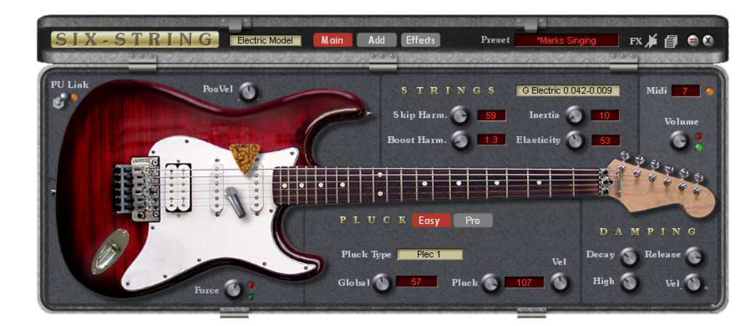
Six-String (SonicCore), an FTM guitar for the SCOPE DSP platform · screenshot © SonicCore
blues
jazz

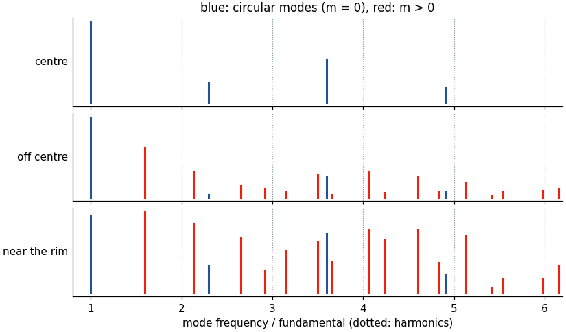
Circular membrane, radius \(a\), fixed rim: modes \(J_m(j_{mn} r/a)\cos(m\theta)\), \[\frac{f_{mn}}{f_{01}} = \frac{j_{mn}}{j_{01}} = 1,\ 1.59,\ 2.14,\ 2.30,\ 2.65,\ \dots\] with \(j_{mn}\) the zeros of the Bessel function \(J_m\): inharmonic, so no clear pitch.
| Same drum, struck | |
|---|---|
| at the centre | |
| off centre, \(0.4a\) | |
| near the rim, \(0.85a\) |
At the centre every mode with \(m > 0\) has a nodal line: only the circular modes ring, a dull thud. The pluck-position slide in 2D: drummers strike off centre.
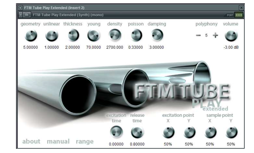
FTM-Tube VST plugin
R. Rabenstein, T. Koch, and C. Popp, Tubular bells: a physical and algorithmic model, IEEE Trans. Audio, Speech, Lang. Process., 2010.
Physical parameters become sound-design knobs, far outside what real tubes can do:
glockenspiel geometry
extreme geometry
damping and excitation sweep
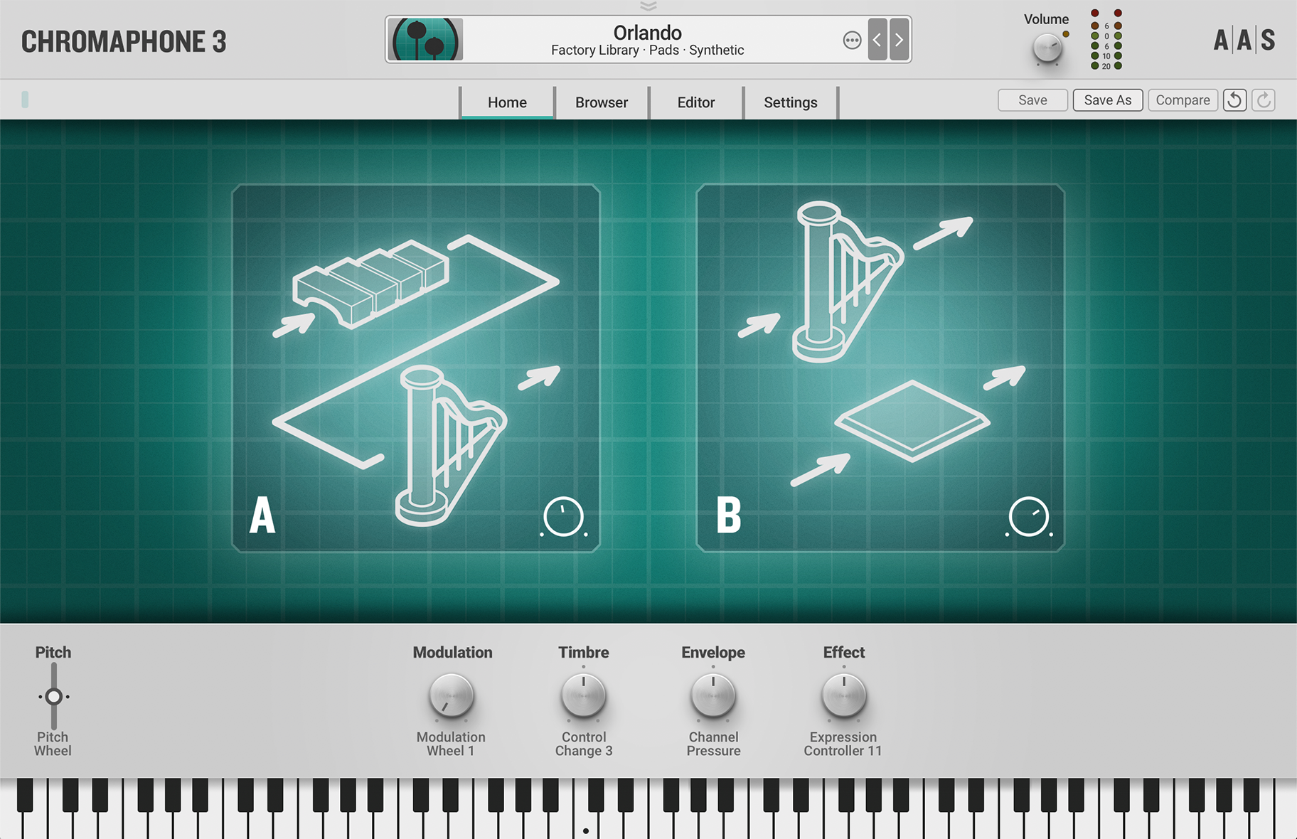
AAS Chromaphone 3: modal resonators (plates, membranes, tubes) excited by mallets and noise
Screenshot © Applied Acoustics Systems
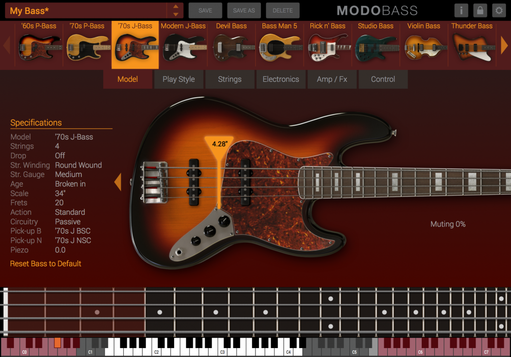
IK Multimedia MODO BASS: modal bass guitar; pluck position, pickups, and strings are parameters
Screenshot © IK Multimedia
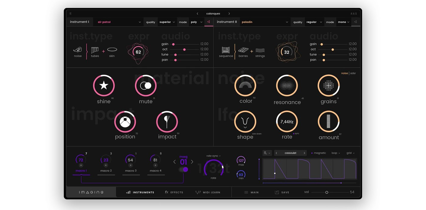
Expressive E Imagine: physical modeling synthesizer plugin
Screenshot © Expressive E
Also: Pianoteq (Modartt), a physically modeled piano whose install is a small fraction of a sampled piano’s, with every string, damper, and resonance adjustable.
| target | |
| lecture 7: additive, ideal string | |
| lecture 7: subtractive | |
| today: modal string |
What is still missing?
And who chose \(B = 5\cdot 10^{-5}\), \(\sigma_0 = 6\), \(x_e = 0.15\)?
Next: fit them
The model is a differentiable function of \((B, \sigma_0, \sigma_2, x_e, x_o, \dots)\). Lecture 10 estimates those parameters from the recording by gradient descent; lecture 11 does the same for a room.
| FDTD | Modal / FTM | Waveguide | |
|---|---|---|---|
| Representation | displacement on a grid | modal amplitudes | two traveling waves |
| Controls | anything in the PDE, input anywhere | \(f_\mu, \sigma_\mu\), excitation and pickup position | loop filter, delay, excitation |
| Built-in structure | local physics, stability limit | linear, decoupled resonators | 1D, lossless core plus filters |
| Fixed vs. learned | derived from physics | derived, or fitted to recordings | derived, or fitted |
One system, three bases
FDTD samples the field, modes diagonalize it, waveguides split it into traveling waves. All three describe the same string; FTM gets the modes without a grid.
The input is a parameter
Excitation shape, position and pickup are vectors \(\mathbf b\) and \(\mathbf c\). Changing how the string is played costs a multiplication, not a new recording.
The same kind of object
A string, a reverb, and later a network layer: large, sparse, recursive state-space systems. Their parameters are physical, and fittable.
New examples in this deck: slides/make_physical_media.py and slides/make_drums_media.py (membrane, KS drum), and the FDTD notebook. String, FTM, VL1 and product media from the LMS/FAU lecture material (slides/make_synthesis_media.py).