Artificial Reverberation

Lecture 11 · Reverb as a controllable dynamical system

Prof. Dr.-Ing. Sebastian J. Schlecht

Where we are

One question, asked of every method

Block	Representation	Generator
Filters and effects	LTI and time-varying systems	hand-designed
Classical synthesis	samples, partials, modes, physical state	hand-designed
DDSP	the same structured models	parameters learned
Reverberation	a recursive dynamical system	hand-designed, fittable
Diffusion	a learned representation	learned

The four questions

How is the sound represented?
What are the controllable parameters?
What structure is built in?
What is fixed by design, and what is learned?

Today, the capstone: reverb is not just an effect you add. It is a small recursive system whose parameters are the things you hear, and it needs every idea of the course so far.

Everything so far, in one room

Lecture	Idea	In a reverb
2–6 (Max)	delay lines, comb filters, Karplus–Strong	the feedback comb, Schroeder
7	modulation, waveshaping	time-varying and nonlinear FDN
8	the recording itself	convolution with a measured room
9	modes, state space	one mode per delay sample
10	parameters fitted by gradients	matching a measured room

Every lecture’s riff, in one FDN room:

7 · additive
9 · modal string
10 · fitted string
the real guitar

Listen

One guitar, six rooms

Dry

Measured room (convolution)

One feedback comb

Schroeder, 1961

Feedback delay network

Time-varying FDN

Listen first

Which ones sound like a room? What exactly is wrong with the others?

What are we actually trying to control?

What you hear	Physical cause
decay time	room volume vs. absorption
damping: highs die first	air and wall absorption rise with frequency
density: smooth, not flutter	many reflections, quickly
color: no ringing tones	many modes, evenly spread
size	early reflection timing
movement	nothing in a static room

Goal of the lecture

A compact recursive system whose parameters map onto the left column, and that costs the same whether the tail is 0.5 s or 10 s long.

Represent

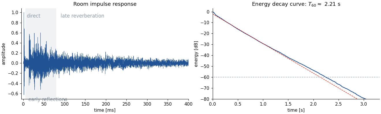
The room impulse response

Direct sound: direction of the source
Early reflections (up to ≈ 80 ms): geometry, size, materials
Late reverberation: reflections too dense to separate; Gaussian noise under an exponential envelope

Energy decay curve (Schroeder 1965)

\[\mathrm{EDC}(t) = \int_t^\infty h^2(\tau)\, d\tau\]

\(T_{60}\): time to fall by 60 dB. Fit a line to −5…−35 dB and extrapolate.

Reverberation time

Sabine’s formula

\[T_{60} \approx 0.161\,\frac{V}{S\,\bar\alpha}\]

volume \(V\) in m³, surface \(S\) in m², mean absorption \(\bar\alpha\). Bigger room, longer tail; more absorption, shorter tail.

The late part of an RIR is almost fully described by \(T_{60}(f)\) and the initial level: a handful of numbers per frequency band.

Speech in four rooms:

classroom
office
lobby
church

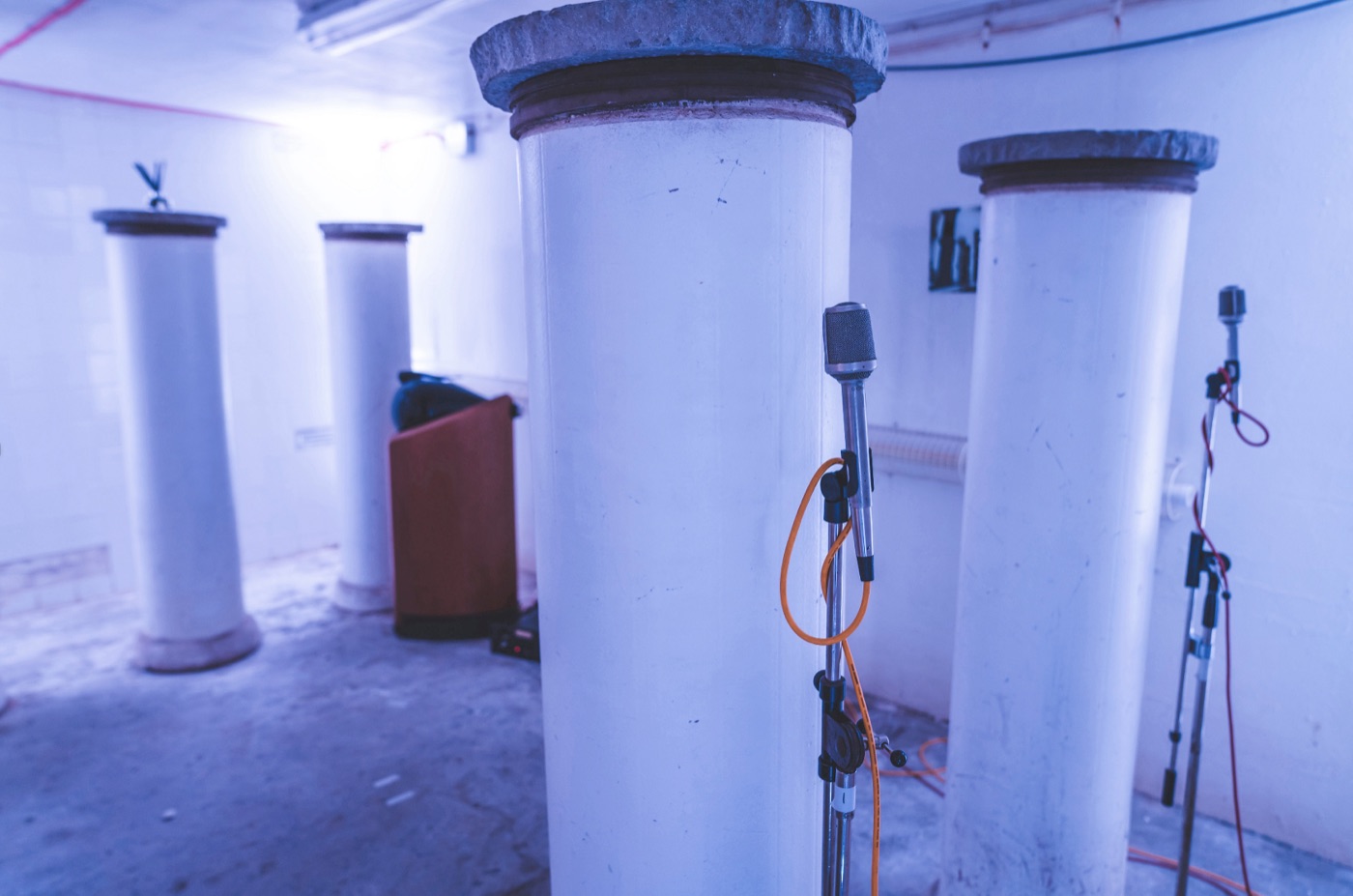
An extreme: 75 seconds of tail

The Inchindown oil tanks in Scotland: a sealed concrete tank, 240 m long, with almost no absorption. Record for the longest reverberation in a man-made structure.

Sabine read backwards: tiny \(\bar\alpha\), big \(V\). The late tail is still just an exponential decay, only a very slow one.

Think

A convolution reverb for this tank at 48 kHz needs how many taps? How many multiplications per output sample?

Before digital: rooms, plates, springs

Echo chamber (Abbey Road): real, not portable.

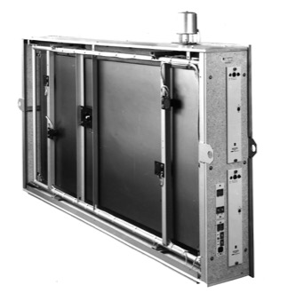
Plate (EMT 140, 1957): steel under tension.

EMT-Archiv-Lahr, CC BY-SA 4.0

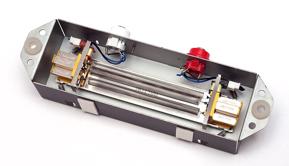
Spring (Hammond, 1941): dispersive chirps.

Ashley Pomeroy, CC BY-SA 4.0

Convolution: exact, but not a model

\[y[n] = \sum_{k=0}^{L-1} h[k]\, x[n-k]\]

Good

reproduces a measured room exactly
FFT and partitioned convolution make it real-time

Not good enough

one room, one source and one listener position
cost and memory grow with \(T_{60}\)
no knobs: “a bit less damping” means re-measuring

The representation we want

Not the impulse response itself, but a small generative model of it: a recursive system with a few parameters that sets \(T_{60}(f)\), density and color.

Structure

The feedback comb, again

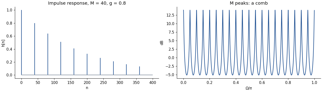
From Max’s delay-line lectures, and Karplus–Strong in lecture 9: \[H(z) = \frac{1}{1 - g\,z^{-M}}\]

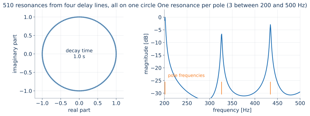
\(M\) poles on a circle of radius \(g^{1/M}\)
decay: \(g = 10^{-3M/(f_s T_{60})}\) gives exactly \(T_{60}\)
cost does not depend on \(T_{60}\)

One delay = echoes every M samples and equally spaced resonances: a flutter, and a pitch.

Schroeder 1961: combs in parallel, allpasses in series

\[A(z) = \frac{-g + z^{-M}}{1 - g\,z^{-M}}, \quad |A(e^{j\Omega})| = 1\]

Combs set the decay and add modes
Allpasses multiply the echoes without coloring the spectrum

impulse train
Schroeder
Moorer (1979): lowpass in each comb

The feedback delay network (Jot & Chaigne 1991)

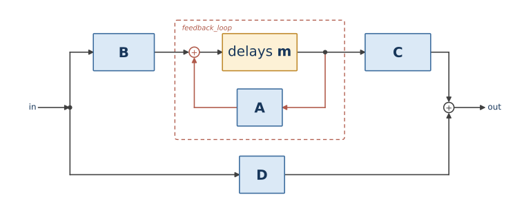
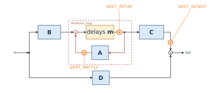
\(N\) delay lines \(m_i\), all feeding back into all through a matrix \(\mathbf{A}\):

\[ \begin{aligned} y[n] &= \mathbf{c}^\top \mathbf{s}[n] + d\,x[n]\\ s_i[n + m_i] &= \textstyle\sum_j A_{ij}\, s_j[n] + b_i\, x[n] \end{aligned} \]

Generalizes the parallel combs (\(\mathbf{A}\) diagonal) and, with the right \(\mathbf{A}\), the whole Schroeder reverberator. Earlier forms: Gerzon (1971), Stautner & Puckette (1982).

An FDN is a state-space system

Transfer function, with \(\mathbf{D_m}(z) = \operatorname{diag}(z^{-m_1}, \dots, z^{-m_N})\):

\[H(z) = \mathbf{c}^\top \big(\mathbf{D_m}(z^{-1}) - \mathbf{A}\big)^{-1} \mathbf{b} + d\]

poles = roots of \(\det\big(\mathbf{D_m}(z^{-1}) - \mathbf{A}\big)\)
there are \(\sum_i m_i\) of them: one mode per sample of delay
8 lines × 2000 samples = 16 000 modes from a 8×8 matrix

Stack every sample in every delay line into one state vector \(\mathbf{x}\):

\[\mathbf{x}[n+1] = \hat{\mathbf{A}}\,\mathbf{x}[n] + \hat{\mathbf{b}}\,x[n]\]

Seen before: the string

It is exactly the form lecture 9 got by discretizing a string or a plate. A reverb and a physical model are the same kind of object: a large, sparse, recursive linear system.

Lossless first, then add loss

Lossless FDN

If \(\mathbf{A}\) is orthogonal (\(\mathbf{A}^\top\mathbf{A} = \mathbf{I}\)), the loop keeps all energy: every pole lies on the unit circle.

Design in two steps:

choose a lossless loop: delays + orthogonal matrix
add loss as a separate, controllable block

That split is what makes the parameters interpretable.

Three reverberators, one family

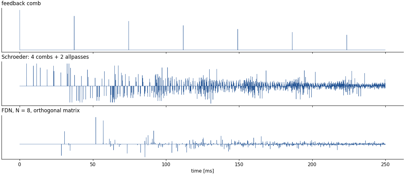
The comb repeats one echo. Schroeder’s allpasses multiply the echoes. The FDN’s matrix makes every echo spawn \(N\) new ones: echo density grows with time, as in a real room.

Control

Knob 1: the delays set size and density

modal density: \(\sum_i m_i / f_s\) modes per Hz
short delays: small, boxy, colored; long delays: large, sparse at the start
coprime lengths, or echoes coincide and ring
physical anchor: the mean free path of the room

Delays
6–19 ms
27–77 ms
52–146 ms

Same decay, same matrix. Only the delays change.

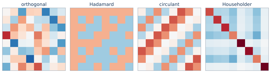
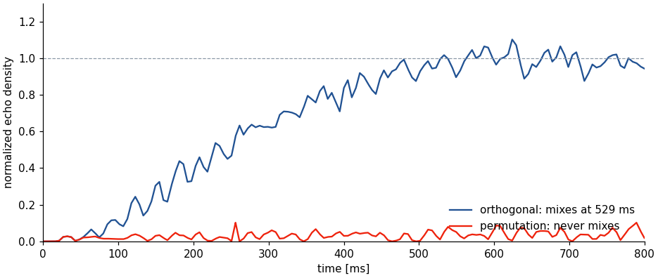
Knob 2: the matrix mixes

Matrix
orthogonal
permutation

Failure case: a permutation is lossless but never mixes. It is one long comb filter.

Knob 3: absorption sets \(T_{60}(f)\)

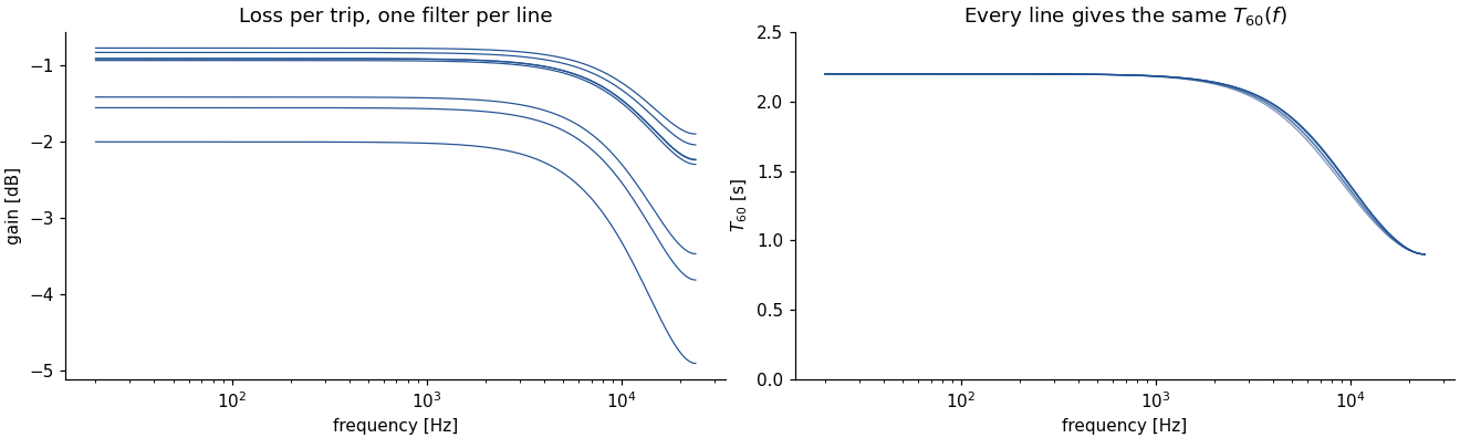
Loss proportional to delay length, so all lines decay together:

\[\gamma_i = 10^{-3 m_i / (f_s T_{60})}\]

Make \(\gamma_i\) a lowpass (Moorer’s idea) and \(T_{60}\) becomes \(T_{60}(f)\).

\(T_{60}\) at Nyquist
0.25 s: dark		2.0 s: bright

Three places to hang a filter

after the delays: absorption, the decay
after the matrix: time variation, nonlinearity (next section)
on the output: tone correction, which colors the reverb without changing its decay

Make it playable

Which knobs would you give a performer?

The FDN has \(N\) delays, \(N^2\) matrix entries, \(N\) absorption filters, \(2N\) gains. A musician wants four.

Macro	FDN parameters behind it
Size	delay range \(m_i\) (and pre-delay)
Decay	\(T_{60}\) at DC, via all \(\gamma_i\) at once
Damping	\(T_{60}\) at Nyquist relative to DC: the absorption filter slope
Mix	\(d\) versus \(\mathbf{c}\)

One macro moves many parameters, and the mapping is designed, not derived. This is the control mapping problem that returns in every synthesis lecture.

Beyond LTI

Time-varying FDN: modes that never sit still

Replace \(\mathbf{A}\) by \(\mathbf{A}[n]\), a rotation that moves slowly:

\[\mathbf{A}[n] = \mathbf{A}\,\mathbf{R}(\theta[n]), \qquad \theta[n] = \theta_0 \sin(2\pi f_m n / f_s)\]

orthogonal at every sample: energy per trip unchanged, so decay and stability are unchanged
no fixed transfer function, so no fixed resonance can ring
related: modulated delay lines (chorus, from Max’s lecture)

static
rotating, 10 Hz

Keep this in mind

Time variation breaks up ringing modes without adding loss. In a few slides it keeps a real concert hall from howling.

Nonlinear FDN: the loop generates new frequencies

Put a nonlinearity after the matrix, on some lines:

\[f(x) = (1-\alpha)\,x + \alpha\,|x|\]

rectification creates harmonics of whatever is ringing
they are fed back, mixed, and rectified again: the effect compounds every trip
shimmer reverbs do the same with a pitch shifter in the loop
the operator must roughly preserve energy, or the tail dies or explodes

linear
half the lines rectified, α = 0.25

No transfer function, no poles, no \(T_{60}(f)\) formula. We can still reason about energy: that is what survives when linearity is gone.

Reverberation enhancement

Make a real room sound bigger

Photo: Gian Marco De Bortoli

Reverberation enhancement system (RES)

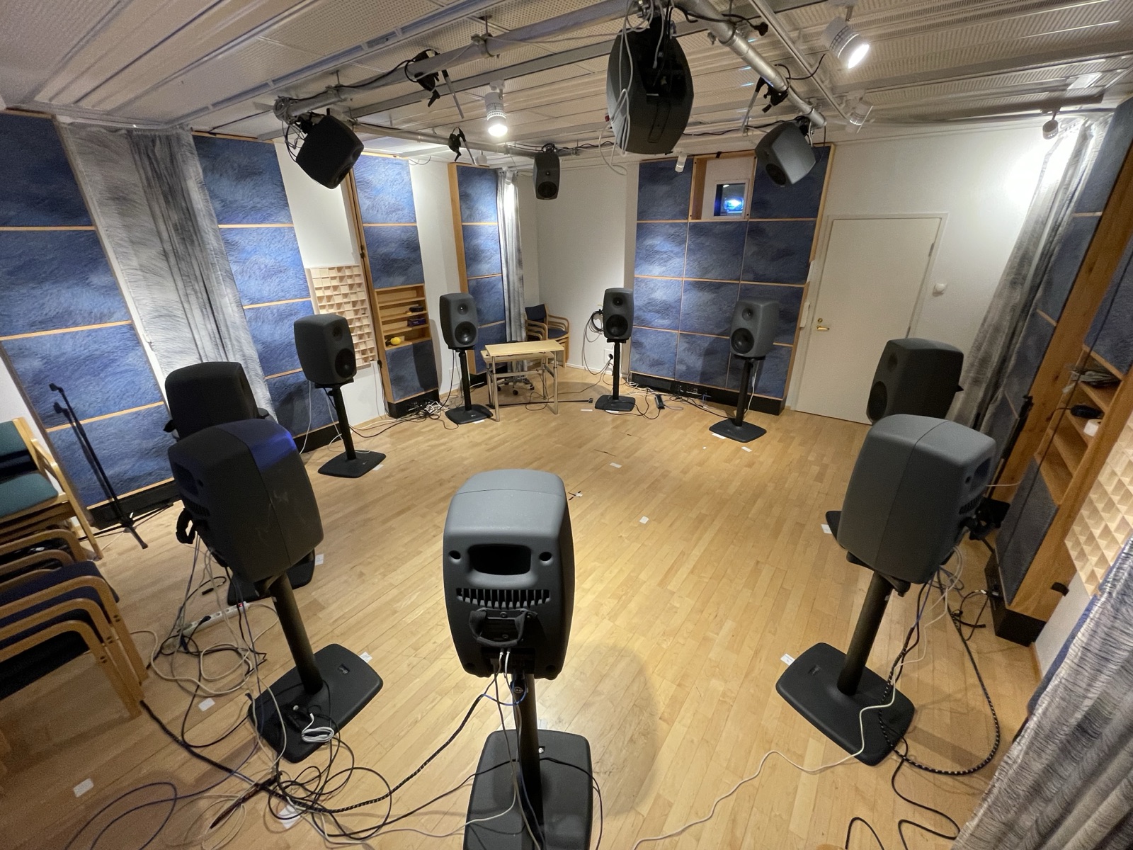
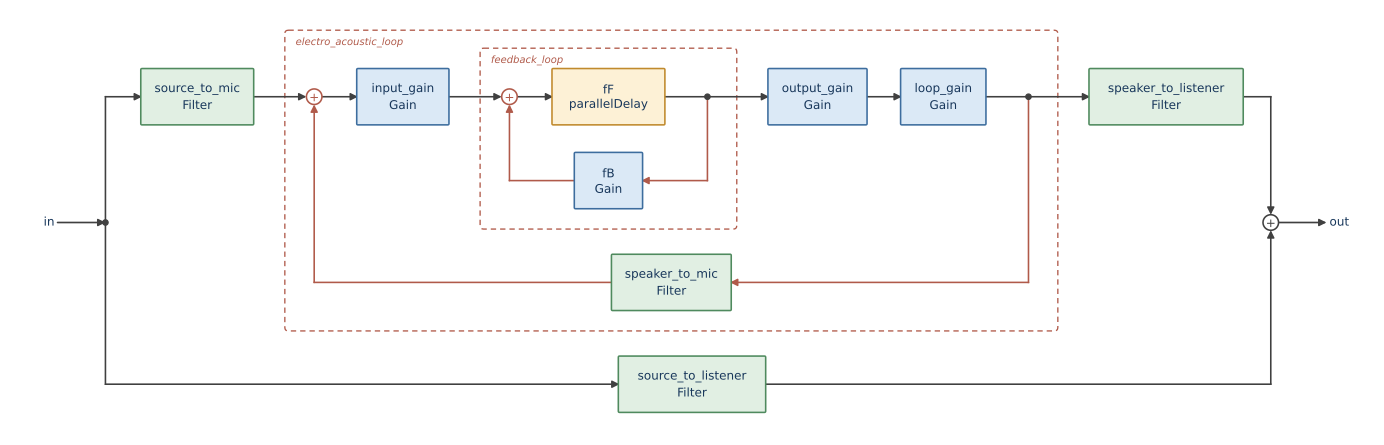
Microphones pick up the room, a reverberator processes the signals, loudspeakers play them back into the same room: electronically variable acoustics.

system off
system on

Multipurpose halls, rehearsal rooms, installations.

Seventy years in five systems

1950s	1964	late 1960s	1990s	2015
Ambiophony (Vermeulen): delayed feeds to loudspeakers	Frequency shifting (Schroeder): break the feedback loop	Multiple-channel amplification of reverberation (Franssen): many weak channels	VRAS (Poletti): an FDN-like reverberator inside the loop	Time-varying FDN (Schlecht & Habets): move the loop itself

Every entry fights the same enemy: the loudspeakers are heard by the microphones.

The room closes the loop

Loudspeakers → microphones: an \(M \times M\) matrix of room responses \(\mathbf{H}(z)\). Reverberator with gain \(G\): \(\mathbf{U}(z)\).

\[\text{closed loop} = \big(\mathbf{I} - G\,\mathbf{U}(z)\,\mathbf{H}(z)\big)^{-1}\]

An RES is an FDN

The room is the feedback matrix, only with long filters instead of scalars. Everything from this lecture applies: mixing, loss, time variation.

Stability: the loop must lose energy

One channel (Nyquist, simplified): stable if

\[|G\,U(e^{j\Omega})\,H(e^{j\Omega})| < 1 \quad \text{for all } \Omega\]

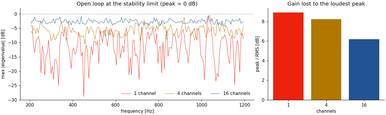
Many channels (Ohsmann 1990): stable if every eigenvalue of the open loop \(G\,\mathbf{U}(e^{j\Omega})\mathbf{H}(e^{j\Omega})\) stays inside the unit circle.

Too much gain:

Coloration comes first

Just below the limit, the loudest peak of the open loop is almost lossless. It rings: the system is stable, but colored.

Two degrees of one artifact

Instability and coloration both come from the peaks of the open loop. Reduce the peaks and you can raise the gain.

More channels, flatter loop

the gain is set by the loudest peak; enhancement comes from the average
more channels sum room resonances incoherently: the peaks stand out less
mixing channels with an orthogonal matrix has a similar effect (Schlecht & Habets 2016)

Time variation raises the stable gain

Frequency shift (Schroeder 1964): shift the loop by a few Hz. A resonance never meets itself on the next trip, so it cannot build up. Fine for speech, audible on music.

Time-varying mixing matrix (Schlecht & Habets 2015): the multichannel version. The same rotating orthogonal matrix as in the time-varying FDN: no added loss, no fixed peaks.

One idea, used twice

In the reverb, time variation stops the modes of the FDN from ringing. In the RES, it stops the modes of the room plus FDN from ringing. Same operator, same reason.

No perfect architecture

Tool	Against	Price
more channels, channel mixing	coloration, instability	hardware
equalization of the loop	peaks in the open loop	must be redesigned when anything changes
feedback cancellation	the loop itself	hard, grows with channel count
time-varying processing	ringing modes	audible if too fast
separate early and late paths	wrong perceived size	design effort

The loop equalizer can be optimized by gradient descent through the whole closed loop (De Bortoli et al., DAFx 2024): lecture 10’s idea, with the real hall inside the loop.

Match

From knobs to a target

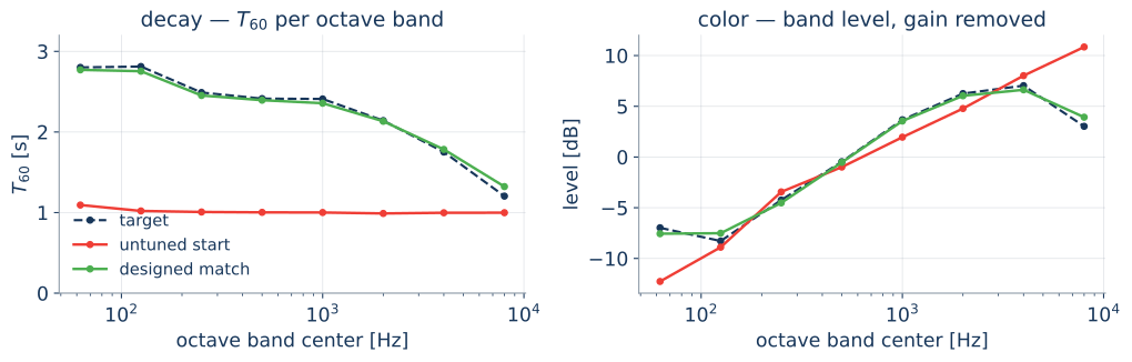
Given a measured room, find the FDN that sounds like it:

\[\hat{\theta} = \arg\min_\theta\ L\big(h_\theta,\ h_\text{target}\big)\]

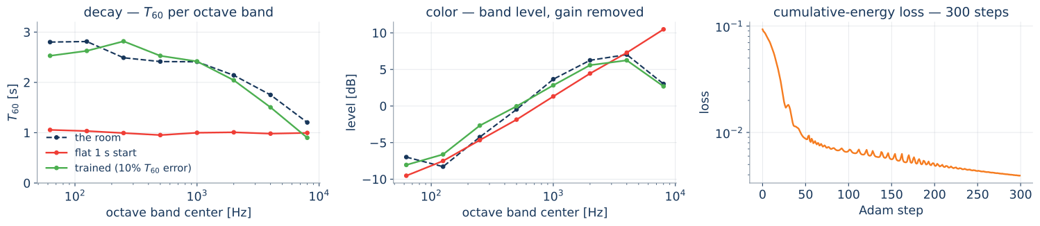
Lecture 10’s method, every FDN block differentiable (FLAMO, pyFDN): delays fixed; absorption, EQ, matrix learned; the loss hears the decay, not the waveform.

target room
FDN, before
FDN, after fitting

Wrap-up

The four questions, for reverb

	Convolution	FDN
Representation	the measured impulse response	the state of \(N\) delay lines
Controls	none	size, decay, damping, mix, modulation
Built-in structure	none: any LTI response	recursive, lossless core plus loss
Fixed vs. learned	measured	designed, then fitted with lecture 10’s method

Take away

A model, not a recording

An FDN is a small recursive system with one mode per delay sample. Its cost does not depend on the decay time.

Parameters you can hear

Delays set size and density, the matrix sets mixing, the absorption filters set \(T_{60}(f)\). Time variation and nonlinearity keep the loop lossless but move or enrich the modes.

The loop can be the room

A reverberation enhancement system is an FDN closed through a real hall. Stability and coloration are the same problem, fought with channels, mixing and time variation.

Every reverberator today was a designed structure with fitted parameters. Lecture 12 drops the structure too: a diffusion model learns the representation and the generator from data.