Samples and Grains

Lecture 8 · Sampling, granular synthesis, and the phase vocoder

Prof. Dr.-Ing. Sebastian J. Schlecht · Dr.-Ing. Maximilian Schäfer

Where we are

One question, asked of every method

Block	Representation	Generator
Filters and effects	LTI and time-varying systems	hand-designed
Classical synthesis	samples, partials, modes, physical state	hand-designed
DDSP	the same structured models	parameters learned
Reverberation	a recursive dynamical system	hand-designed, fittable
Diffusion	a learned representation	learned

The four questions

How is the sound represented?
What are the controllable parameters?
What structure is built in?
What is fixed by design, and what is learned?

Last lecture: write the spectrum down. Today: keep the recording itself, and find out how much control we can get back by cutting it into pieces.

Listen

One recording, five instruments

The guitar riff from lecture 7
played back
four times slower, same pitch
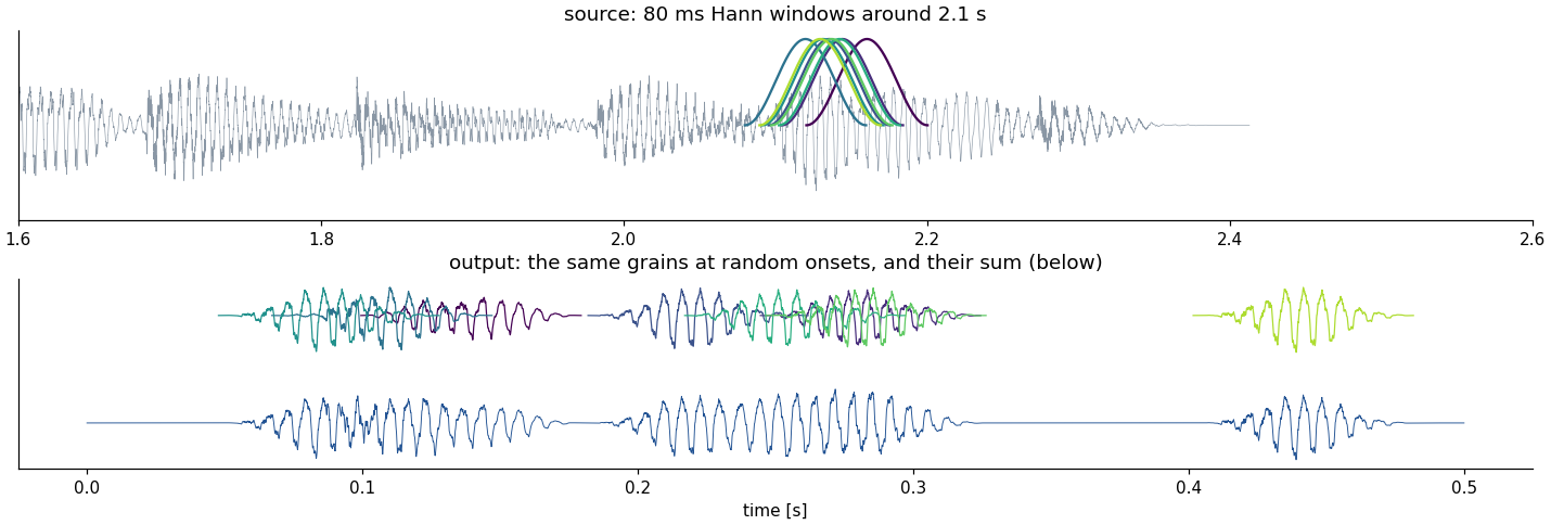
frozen at 2.1 s
scrubbed back and forth
a cloud, in octaves and fifths

Listen first

Every sound on the left is made only of pieces of the first one. Which parameter changes from row to row?

From event to material

Sampling treats a recording as one event to replay. Granular synthesis treats it as a material to navigate: position, speed and pitch become separate controls.

Three ways to cut up a recording

Representation	Unit	What you control
the recording (sampling)	a whole note, seconds long	which note, loop points, playback rate
grains (granular)	windowed pieces of 10–200 ms	position, density, duration, pitch, randomness
STFT frames (phase vocoder)	grains with a Fourier transform: magnitude and phase per bin	time and pitch separately

Down the table, the pieces get smaller and the representation gets more structured, and more can be changed without destroying the sound.

Represent: the recording

Sampling: record once, replay forever

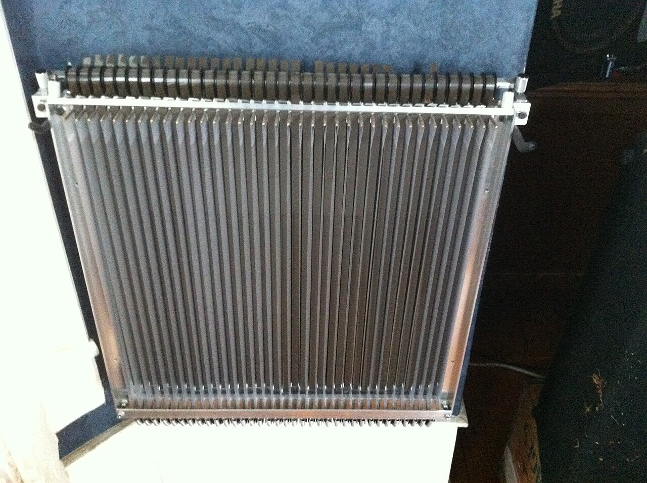
Mellotron, 1963: one tape strip per key · 120years

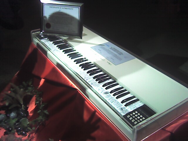
Fairlight CMI, 1979 · 120years

1963, Mellotron: 8 s of tape per key, no loops
1979, Fairlight CMI: digital recording, pitch shifting, looping
1980, Linn LM-1: a drum machine that plays recorded drums
1984, Kurzweil K250: a recording every few keys, a convincing piano
today: tens of gigabytes per instrument

A recording is one performance: one duration, one pitch, one way of playing it.

Failure case: a loop that clicks

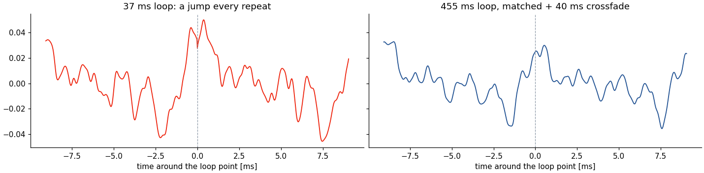
Store 2 s of a piano note (A2), play 6 s:

stored, 2 s
37 ms loop
455 ms loop, matched
the real note

a short loop: a buzz at the loop rate (27 Hz) and a jump per repeat
match end to start (correlation), then crossfade
a decaying note must keep decaying: flatten the loop, apply a decay
left over: the loop freezes the timbre; the real piano gets duller

Pitch shifting: read the table faster

Asynchronous (until ≈1985)

Change the DAC clock per voice. Any pitch, simple circuit, but every voice needs its own converter and all mixing happens in analog.

Synchronous (today)

One sample rate. A phase accumulator advances by a fractional increment, e.g. one semitone: \(2^{1/12} = 1.0595\). The integer part addresses the table, the fraction interpolates.

Speech, read \(2^{5/12}\) times faster:

original
a fourth up

Pitch, duration and formants all move together: the chipmunk.

That is why samplers store a new recording every few semitones.

Interpolation you can hear

A short 64-sample sawtooth table, played one semitone above A4.

Drop-sample (order 0): every 17th sample repeats

Linear (order 1)

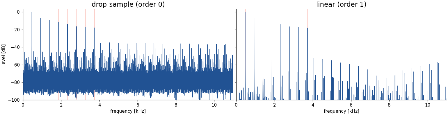
Red lines: the eight harmonics that should be there. Everything else is interpolation error that aliases back as inharmonic noise: lecture 7’s failure case, from a different cause.

Multisampling: memory for variability

Stop pitch shifting and looping: record every key, every velocity, every playing style.

A grand piano, the old estimate

88 keys × 8 velocity layers × 2 minutes ≈ one day of audio, about 1.8 GB. Only the start of each sample sits in RAM; the rest streams from disk.

Today’s sampled pianos add round-robins, pedal resonance, release noises and several microphone positions: tens of gigabytes per instrument is normal.

The price is still variability: the sampler cannot play what nobody recorded, e.g. a half-pressed pedal or a string that is already ringing.

Structure: grains

Granular synthesis: many short windows

\[y(t) = \sum_k w(t - t_k)\; x\big(p_k + r_k\,(t - t_k)\big)\]

grain \(k\): onset \(t_k\), read position \(p_k\), playback rate \(r_k\), window \(w\)

overlap-add: grains that overlap sum to a continuous sound
the window removes every click at once: no loop points to find
10–200 ms: long enough to keep pitch, short enough to rearrange

Grain parameters are performance controls

Parameter	Effect	The listening examples
position \(p(t)\)	where in the recording	advance slowly: stretch. Stop: freeze. Sweep: scrub
playback rate \(r\)	pitch of each grain	½, 1, 3/2, 2: the cloud’s chord
density	grains per second	sparse: rhythm and glitch. Dense: a smooth texture
duration	grain length	short: noisy, pitch lost. Long: the source shows through
jitter	randomness in all of the above	removes the comb-filter buzz of regular grains

Position and pitch are independent now: that is the whole trick. Time-stretching, freezing, pads from a single note, glitch rhythms, morphing between recordings.

Structure: the phase vocoder

STFT frames are grains with a Fourier transform

\[X(m, k) = \sum_n x[n]\, w[n - mH_a]\, e^{-j 2\pi k n / N}\]

frame \(m\) every \(H_a\) samples, bin \(k\)
magnitude \(|X(m,k)|\): how much of frequency \(k\)
phase \(\angle X(m,k)\): where in its cycle it is

Stretch time: read frames at hop \(H_a\), write them at hop \(H_s > H_a\).

Failure case: just move the frames

Each frame keeps its original phase. Neighbouring frames no longer line up, and their overlap cancels and beats.

1.8 × longer
frames moved (OLA)
phase vocoder

The phase vocoder: advance each phase at its true frequency

Bin \(k\) expects a phase advance of \(\omega_k H_a\) per frame. The measured deviation reveals the true frequency of the partial in that bin:

\[\hat{\omega}_k = \omega_k + \frac{\operatorname{princarg}\big(\angle X(m{+}1,k) - \angle X(m,k) - \omega_k H_a\big)}{H_a}\]

Then write the output with that frequency and the new hop:

\[\varphi(m{+}1, k) = \varphi(m, k) + \hat{\omega}_k H_s\]

Measured on the speech example, median pitch:

	\(f_0\)
original	203 Hz
frames moved (OLA)	174 Hz, smeared
phase vocoder, 1.8 × longer	203 Hz

Flanagan & Golden, Bell Labs, 1966; Dolson’s tutorial (1986) brought it to music.

Pitch without time, and what still goes wrong

Pitch shift = stretch by \(r\), then resample by \(r\): same duration, pitch × \(r\).

A fourth up
resampled: shorter
phase vocoder: same length

Measured: 203 → 271 Hz, ratio 1.334 (target \(2^{5/12} = 1.335\)).

Still wrong

formants move with the pitch: still a chipmunk. Fix: separate source and filter (lecture 7), shift only the source
transients get smeared over a frame: drums go soft
phasiness: partials in neighbouring bins drift apart. Fix: lock their phases together (Laroche & Dolson 1999)

Only the magnitude

Throw the phase away. What is left?

Keep \(|X(m,k)|\) only, and invent a phase:

original
zero phase
random phase
Griffin–Lim, 100 iterations

Griffin–Lim (1984)

Alternate: take the phase of the STFT of the current signal, put the target magnitude back, invert. Converges to a signal whose magnitude matches.

Spectral error \(\| |X| - |\hat X| \| / \| |X| \|\): random phase 0.54, Griffin–Lim 0.06.

A consistent magnitude is not the original: the phase that made the voice sound alive was never in the magnitude.

Neural vocoders: learn the missing part

Most modern speech and music generators do not output a waveform. They output a mel spectrogram: magnitude only, on a coarse perceptual frequency scale.

\[M(m, b) \;\longrightarrow\; f_\theta(M) \;\longrightarrow\; x[n]\]

The vocoder \(f_\theta\) is a network that learned what waveform is likely to have produced \(M\). Autoregressive (WaveNet, 2016), adversarial (HiFi-GAN, 2020), diffusion (lecture 12).

	Channel vocoder (L7)	Neural vocoder
representation	band envelopes	mel spectrogram
generator	carrier + filters	learned network
missing information	filled by design	filled from data

The question for every representation

What does it keep, and what must the generator infer?

Control

Failure case: the machine gun

One drum hit, 24 times in a row:

the hit
identical copies
each copy slightly different

Per hit: a new velvet-noise filter (8 random-sign taps in 4 ms) on a low-shelved copy, added 14 dB below the dry hit (Fagerström et al. 2021); plus accents and ±2 ms timing.

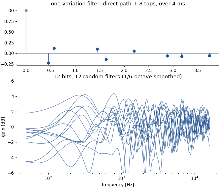
No drummer hits twice the same way. Samplers answer with round-robins (several recordings per note) or, as here, with variation synthesis: small random processing that the ear reads as a new stroke.

Drum machines hit this first: the LM-1 (1980) played one sample per drum, and the machine gun is how early sampled drum tracks give themselves away. A synthesized drum (the 808, lecture 7) gets some variation for free: its noise and free-running oscillators never start the same way.

Make it playable

Which knobs would you give a performer?

A granular instrument has position, rate, density, duration, jitter, window shape, and a source. A performer gets three.

Macro	What moves behind it
position (a fader or a touch strip)	\(p(t)\), with a small jitter always on
pitch spread	the set of playback rates, and how randomly they are chosen
texture	density and duration together: from sparse clicks to a smooth pad

The same pattern as the FM index in lecture 7: one perceptual knob moves many parameters.

Match

The perfect match, with nothing to play

Sampling matches the target exactly: the recording is the target. Every step since has traded some fidelity for some control:

	Fidelity	Control
playback	perfect	none
loop, resample	good	length, pitch (with formants)
granular	the texture survives	position, pitch, density
phase vocoder	good, smeared transients	time and pitch separately
lecture 7: additive / subtractive	far	many, meaningful

What none of them has

A reason. Pluck the same string harder, or at another position, or while it still rings: a recording cannot answer, and neither can a filtered sawtooth.

Next lecture models the mechanism: the string itself. Then every one of these questions becomes a parameter.

Wrap-up

The four questions, for samples and grains

	Sampling	Granular	Phase vocoder
Representation	the recording	windowed grains	STFT magnitude and phase
Controls	note, loop, rate	position, rate, density, duration, jitter	time and pitch separately
Built-in structure	none	overlap-add	sinusoids with a true frequency per bin
Fixed vs. learned	recorded	recorded, rearranged	analysed; the magnitude-only case is learned by neural vocoders

Take away

Recording as material

Loops, grains and frames cut a recording into pieces small enough to rearrange: sustain, time stretch, freeze, clouds.

Time and pitch, separated

Resampling couples pitch, duration and formants. The phase vocoder decouples time and pitch by advancing each bin at its true frequency; formants need a source-filter split.

Keep, or infer

Magnitude-only representations lose the phase. Griffin–Lim finds a consistent one; neural vocoders learn a plausible one.