Feedback Delay Networks in Python

From Theory to Differentiable Design with pyFDN

Sebastian J. Schlecht

Friedrich-Alexander-Universität Erlangen-Nürnberg

Facundo Franchino

Massachusetts Institute of Technology

1 September 2026

Ninety minutes, six moves

Time		Segment	You will…
0:00	15	What is an FDN?	read the block diagram, and where filters go in it
0:15	15	pyFDN, the tour	know where everything lives, run five lines
0:30	10	What to do next?	see where the research frontier is
0:40	25	Hands-on 1 — build one	delays, matrix, gains, decay — then match a hall
1:05	20	Hands-on 2 — match a room	fit one to a measured hall, by gradient descent
1:25	5	Q&A	ask your questions

Slides and setup instructions: artificial-audio.github.io/pyfdn-tutorial-2026

1 · What is an FDN?

A room, one ray at a time

A room, as a signal flow

What an FDN is good at, and what it is not

Strengths

• parametric by design — decay, color and density are knobs, not samples
• cost is independent of the decay time
• one FDN per room, shared by all sources and receivers
• time-varying design is cheap
• small and differentiable, so it can be optimized

Limitations

• it approximates a room, it does not reproduce a measured one
• early reflections are not placed, they need their own stage
• a badly chosen matrix or delay set rings and colors the tail
• the parameters map to what you hear only indirectly

Used in modern frameworks

MPEG-I Immersive Audio

The vanilla structure

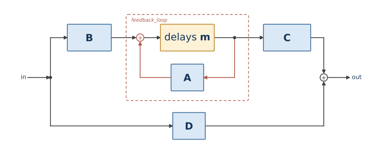
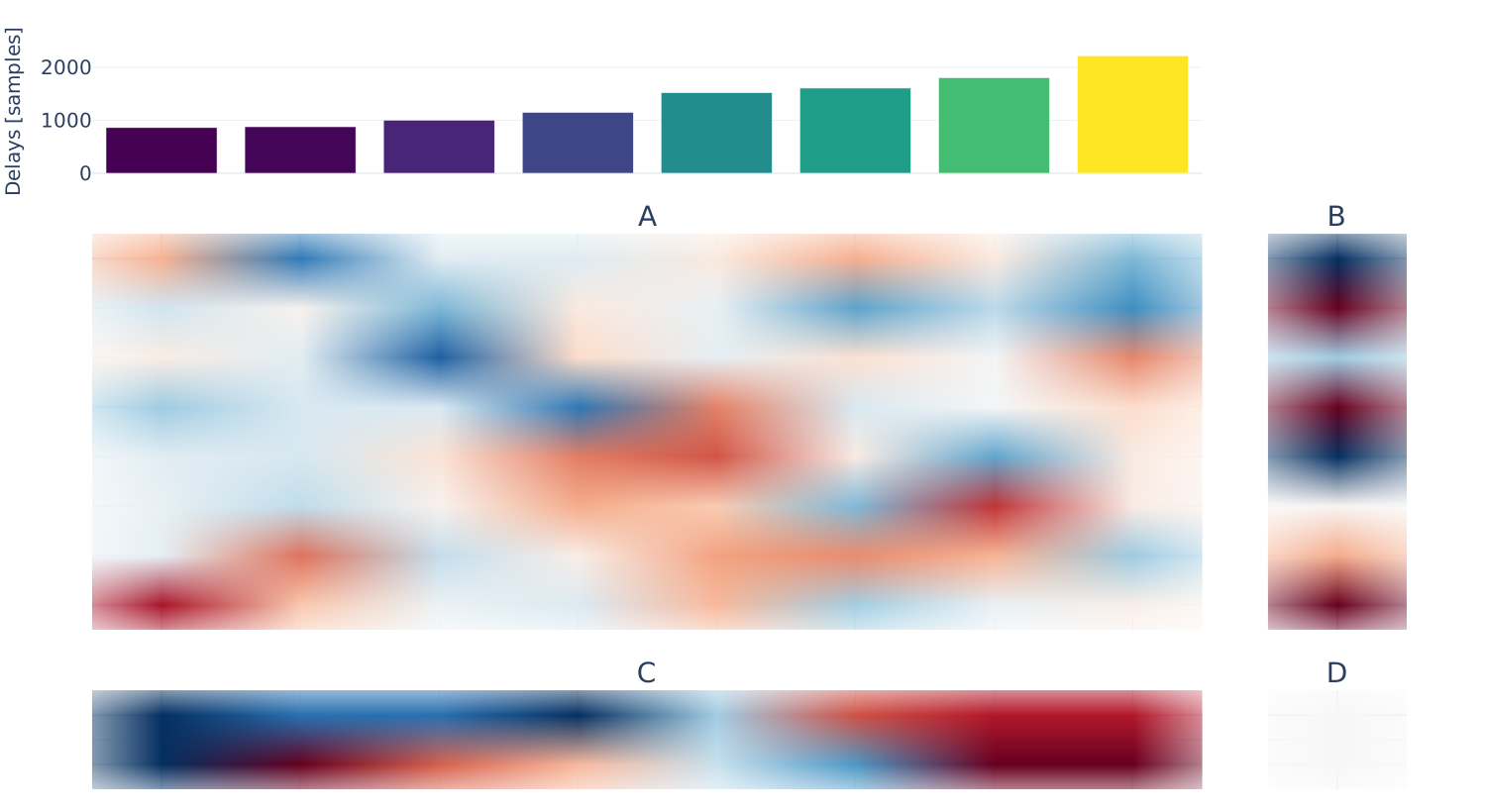
Input gain B, a bank of \(N\) delays, the feedback matrix A, output gain C, and the direct path D around all of it. Four blocks and a loop — that is the whole vanilla FDN.

One FDN, the core parameters

Three places to hang a filter

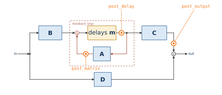
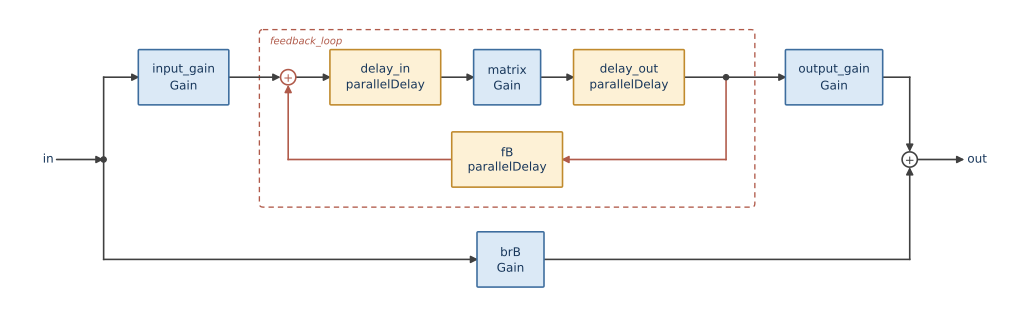
Same structure, three hooks added: the points where pyFDN.process_fdn will take an arbitrary filter — the openings every later structure in this tutorial goes through.

No hooks — the lossless loop

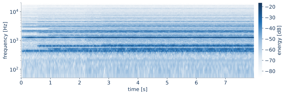
Nothing in the loop but the orthogonal matrix A: energy goes round without being lost. Every hook that follows is a way of taking that energy back.

post_delay — absorption

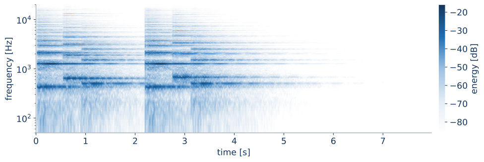
One shelving filter per delay line, \(T_{60}\) of 3.5 s at DC falling to 1.2 s at Nyquist. Watch the top of the spectrogram empty out first — that tilt is the absorption.

post_output — output EQ

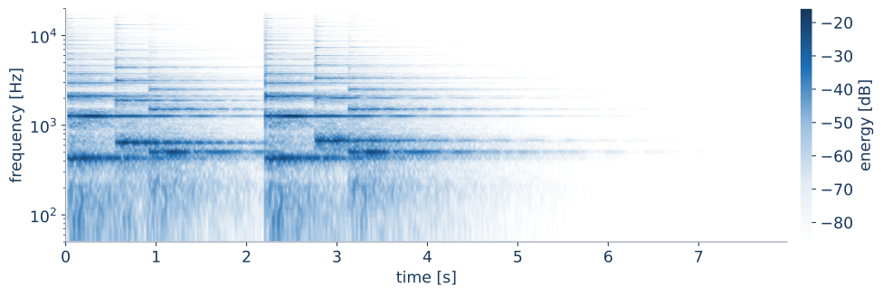
A 10-band gain_to_geq voicing on the wet signal only: \(+5\) dB low, \(-14\) dB at Nyquist. It changes the color of the reverb without touching the decay — the tail is still 3.5 s long.

post_matrix — time-variation

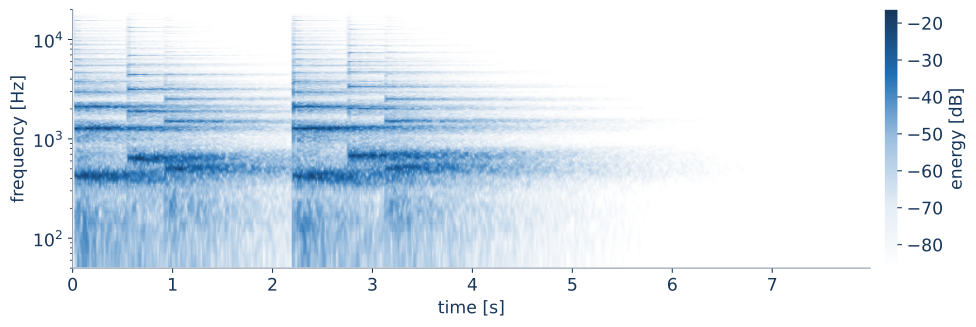
td.TimeVaryingMatrix(N, 10 Hz, 1.1 rad, fs, spread=0.7) — the same hook, but the matrix moves. Orthogonal at every sample, so the decay is unchanged.

post_matrix — a non-linearity

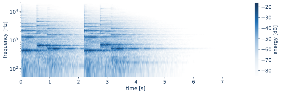
post_matrix=td.ControllableFullWaveRect(N, 0.25, [4,5,6,7]) — half the lines partly rectified. alpha runs from untouched to a full-wave rectifier, so it turns up live. The harmonics were never in the input; the FDN is generating them, and there is no transfer function left to plot.

→ One of six shimmer operators new in pyFDN 0.4.2 — Dal Santo et al., Shimmer Reverberation with Nonlinear FDNs, at this conference.

Beyond the vanilla FDN — toward arbitrary structures

Three connectors, in both backends (td.Series / flamo.Series, …). The vanilla FDN is one Recursion inside a Series inside a Parallel — nothing in the library says “FDN”.

• Put the mixing chain in the forward path → early reflections
• Put an FDN inside the forward path of another → allpass FDN
• Let the feedback path be a measured room → reverberation enhancement

Early reflections — transpose the recursion

• A short delay → matrix → short delay chain in the forward path; only the long delays recirculate
• Buys echo density early, where a vanilla FDN is still sparse — early-reflection control without a separate FIR stage

Allpass — an FDN inside an FDN

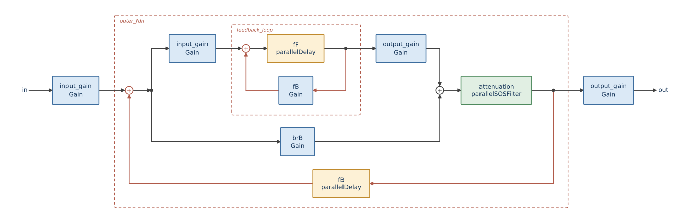
Two nested recursions. The inner loop is a homogeneous MIMO allpass FDN; it and the absorption filter form the forward path of the outer loop, whose feedback path is the main delay bank.

With only 4 main delays:

Reverberation Enhancement System — the room closes the loop

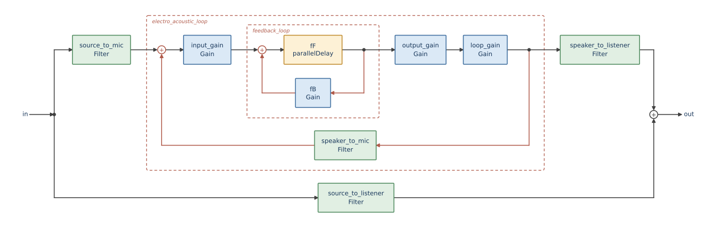
Microphones feed the FDN, the FDN feeds the loudspeakers, and the room’s loudspeaker-to-microphone responses are the feedback path.

So what is actually hard?

• Choosing and comparing structures
• Deriving parameters for these structures (from physics, perceptual features, reference signal or intuition)
• Evaluating consistently and against fair baselines (objectives, complexity, quality)
• Presenting audible and reproducible results transparently

2 · pyFDN, the tour

A toolbox turns FDNs into a shared laboratory

For research

• compare structures through one representation instead of rewriting plumbing
• reproduce figures, listening tests and optimization runs from executable code
• move between time, frequency, modal and differentiable views without changing the underlying design
• turn a paper into a tested constructor, translator or objective that others can extend

For education

• connect the DSP objects students know — delays, filters, poles and matrices — to something they can hear immediately
• expose failure modes: coloration, slow mixing and unstable optimization
• bridge DSP analysis with DDSP design: derive what has a closed form, then optimize what does not
• make every exercise inspectable, editable and repeatable

marimo keeps an experiment and its explanation in sync

What it is

marimo is an open-source reactive Python notebook.

• notebooks are ordinary .py files
• cells form a dependency graph
• changing a value reruns its dependents, or marks them stale
• the same file can run as a notebook, script or web app

Why we use it here

• no hidden “which cell did I run?” state during a live tutorial
• a slider can drive the delays, matrix or decay and update every downstream plot and audio player
• Git diffs and code review stay readable
• examples run in CI and render to a browser-friendly gallery
• one artifact serves teaching, research and documentation

marimo edit examples/     # explore and modify
python example.py         # reproduce non-interactively

Design principles

Functions, not a framework

• flat namespace: everything is pyFDN.<thing>
• NumPy in, NumPy out
• no session object, no builder to learn

Torch only where it earns its place

• analysis and design: pure NumPy/SciPy
• differentiable models: FLAMO (PyTorch)
• one translator between the two: dss_to_flamo

Reference-tested

• ported from the MATLAB FDN Toolbox, with .mat reference fixtures asserting parity
• every example notebook runs in CI
• the API reference cannot silently drift

Notebooks are the documentation

• ~30 marimo notebooks, rendered into the website
• each one is a real .py file — diffable, testable, importable

Open the examples gallery — every one of these is rendered with its outputs and audio.

Three backends, one interface

	process_fdn	td	FLAMO
What it is	the FDN recursion, hard-coded	a graph of block operators	torch.nn.Modules
Domain	time, block-wise	time, block-wise	frequency (FFT)
Structure	vanilla + three hooks	anything you can wire	anything you can wire
Gives you	no dependencies, fast to reason about	streaming, time-varying, non-linear	gradients
Costs you	one topology	no gradients	torch, and an LTI assumption

Same vocabulary in all three: Series, Parallel, Recursion, and a block-processing object with a .filter(block) method.

FDNBuild is what moves between them — design in one, render in another, train in the third, and it is the same FDN.

The map

Module	What is in it	Typical entry points
generate	matrices, delays, allpass, scattering, SDN	fdn_build_gallery, fdn_matrix_gallery, filter_matrix_gallery, sample_delay_lengths, random_orthogonal
process	the FDN recursion in plain NumPy	process_fdn
td	stateful block-processing graph — no torch, no FFT	td.Series, td.Recursion, td.SOSBank, td.MatrixFIR, td.TimeVaryingMatrix
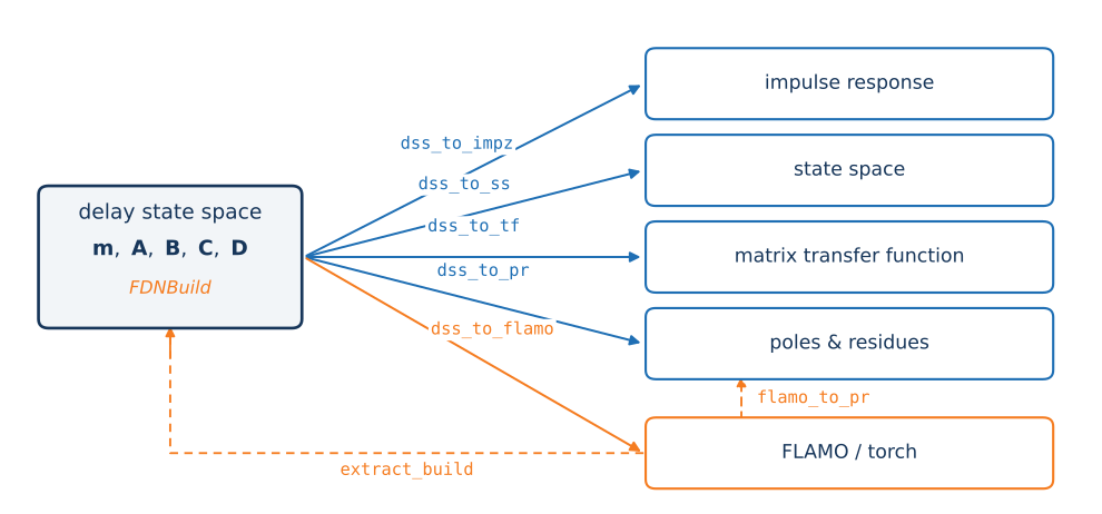
translate	representation changes	dss_to_flamo, dss_to_impz, dss_to_pr, dss_to_ss, dss_to_tf, flamo_to_pr
train	differentiable optimization	build_fdn, train_fdn, Trainable, build_set_decay, extract_build
eq	absorption & equalization filter design	decay_to_geq, gain_to_geq, decay_to_one_pole, EQDesign
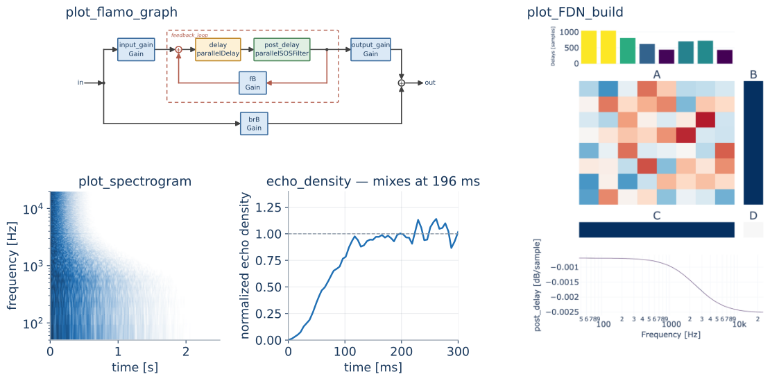
auxiliary	acoustics, math, plotting, FLAMO glue	estimate_rt_bands, echo_density, plot_edc, plot_flamo_graph, flamo_process
presets, build_io	trained FDNs on disk, and your own	load_fdn_preset("colorless_N8_d1"), save_fdn_build
resources	packaged test signals and the bibliography	load_audio("synth_dry"), paper_link

One data class holds an FDN

build = pyFDN.fdn_build_gallery(
    8,                      # eight delay lines
    fs=48_000,
    rt=2.0,                 # T60 at DC
    rt_nyquist=0.5,         # T60 at Nyquist → per-line absorption filters
    io_type="ones",
    rng=42,
)

build.delays    # (N,)              delay lengths in samples
build.A         # (N, N)            feedback matrix
build.B         # (N, n_in)         input gains
build.C         # (n_out, N)        output gains
build.D         # (n_out, n_in)     direct path
build.post_delay   # (n_sos, 6, N)     per-line absorption, or None if lossless
build.post_matrix  # (n_sos, 6, N)     a filter in the feedback path, or None
build.post_output  # (n_sos, 6, n_out) output equalization, or None

FDNBuild is the common currency: every constructor returns one, every translator accepts one, and extract_build(model) gets one back out of a trained model.

Five representations, one hub

A reverb in five lines

import numpy as np, pyFDN
from pyFDN import td

build = pyFDN.fdn_build_gallery(8, fs=48_000, rt=1.8, rt_nyquist=0.4, rng=0)
dry, fs = pyFDN.load_audio("synth_dry")
wet = pyFDN.process_fdn(
    np.pad(dry, (0, 2 * fs)),                       # room for the tail
    build.delays, build.A, build.B, build.C, build.D,
    post_delay=td.SOSBank(build.post_delay),        # the absorption the gallery designed
)

Visualize the model and the build

From design to real-time — arrays to a plugin

Everything so far is offline: Python, torch, FFT-domain recursion. None of it runs in a DAW. adac closes that gap — it walks the FLAMO graph and emits FAUST.

import adac

config = adac.flamo_to_json(model, fs, name="PyFDNReverb")   # graph → JSON IR
cert   = adac.certify(config)                                # stability certificate
faust  = adac.json_to_faust(config, controls={"rt60": True, "dry_wet": True})

From there: the FAUST web IDE, faust -o cpp, faust2juce, or adac.export_juce for a VST3. pip install adac — NumPy only.

Open example_fdn_to_faust in the examples gallery — the same three calls, with the emitted FAUST source rendered underneath.

Franchino & Schlecht, Compiling Differentiable Audio Graphs to Real-Time DSP, DAFx 2026 (arXiv:2606.21277)

3 · What to do next?

The frontier, with notebooks

Direction	Idea	Notebook
Allpass FDNs	uniallpass conditions; nested/series/Poletti structures	example_allpass_FDN_*
Paraunitary	filter feedback matrices; delay & velvet-noise matrices	example_paraunitary_fdn
Scattering	scattering matrices in the loop, more mixing per multiply	example_scattering_fdn
SDN	scattering delay networks — geometry-driven	example_sdn
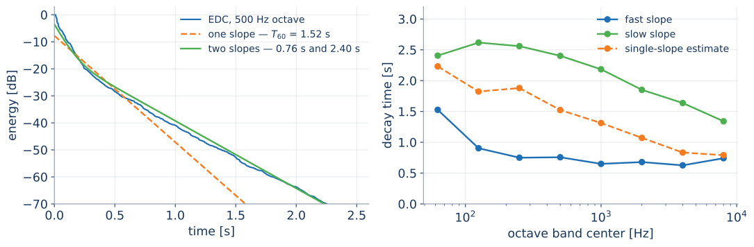
Coupled rooms	multi-slope decay, non-exponential EDCs	example_coupled_rooms, example_multislope_rir_to_fdn
Time-varying	modulated matrices, stability under modulation	example_time_varying_fdn
Shimmer	rectifiers, ring modulation and pitch shifting in the loop	example_shimmer_fdn
Modal analysis	poles, residues, modal excitation, pole spreading	example_dss_to_pr_*, example_spread_fdn_poles
Decorrelation	multi-output FDNs for spatial rendering	example_decorrelation
Real time	compile a design to FAUST, JUCE, a VST3	example_fdn_to_faust

DecayFitNet is now a pip install

pip install multislope

import multislope

net = multislope.DecayFitNet(sample_rate=fs)
fit = net.estimate(rir)             # per octave band

PyPI · source · MIT

DecayFitNet is by Georg Götz, with Sebastian J. Schlecht and Ville Pulkki.

Open research questions

• ‘best architecture’ for a given room — how to choose delays, matrix, and sub-structure
• perceptual objectives — what is the right loss
• differentiable delay optimization — what loss?
• differentiable time-domain optimization
• positional, directional and dynamic scenes
• using the early reflections of the FDN
• conditional generation (using speech, music, text or a room embedding to derive the FDN parameters)

How to contribute

As a developer

Help maintain and stabilize.

• take an open issue — backends, filters, config files, real-time paths
• tests, docs, packaging and CI count as much as DSP
• review pull requests; we need more eyes than hands

As a student

Pick a project off the reverb list.

• issue #123 collects project-sized topics: spring and plate reverb, SDN, velvet noise, binaural FDNs, fade-in FDNs, echo density …
• each one lands as a new .py notebook in examples/
• good scope for a semester project or a thesis chapter

As a researcher

Help integrate your research.

• bring your method in as a hook, not a fork
• a reference implementation inside pyFDN gets used, compared and cited
• talk to us early — the API can bend toward your structure

All of it happens in the open at github.com/artificial-audio/pyFDN — take an issue, or open one.

4 · Hands-on 1 — build an FDN

Open the starter notebook before we begin

A — molab in your browser (recommended)

1. Create an account or sign in at molab.marimo.io
2. Open the pyFDN starter notebook
3. Choose Fork to put an editable copy in your workspace
4. Start the runtime and run all cells once

Do this before the tutorial. Nothing needs to be installed locally.

B — local Python (optional)

uv venv --python 3.11
source .venv/bin/activate
uv pip install "pyfdn[examples]"
git clone https://github.com/artificial-audio/pyFDN
cd pyFDN
marimo edit examples/

import pyFDN
print(pyFDN.__version__)

torch via flamo is the large download, and only Hands-on 2 needs it. Do this before arriving.

Fallback: every notebook is also rendered in the pyFDN examples gallery.

The plan

One notebook, examples/example_process_fdn.py, five steps — three knobs and the wiring between them:

1. Delays (knob 1) — choose the lengths, hear the density
2. Matrix (knob 2) — swap the feedback matrix, measure the mixing
3. Gains — wire the input and output, and render your first impulse response; a second row of output gains makes it stereo
4. Decay (knob 3) — prescribe \(T_{60}\) per band, then check you got it
5. Analyze and listen — EDC, echo density, spectrogram, and your own ears

Open example_process_fdn.py in marimo now and run all cells. Everything in this section is plain NumPy — no torch, no FLAMO. Every code cell ends with a Try this block; that is where the exercises live.

Knob 1 — the delays set the density

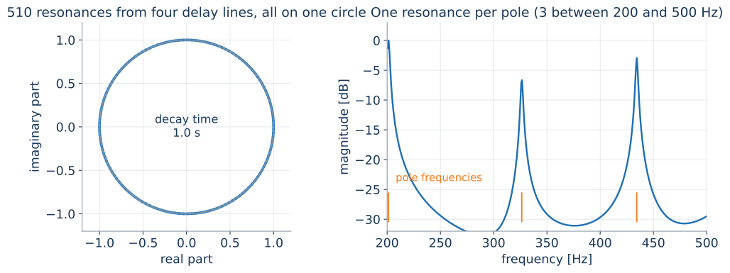
• each delay line adds its own set of resonances — longer delays, more of them
• together they set the density: short delays sound like a small box, long ones like a sparse, granular hall
• echo density builds up over time, faster the more lines you have
• lengths sharing a common factor make echoes coincide — the metallic ring; coprime lengths avoid it
• physical anchor: the mean free path of the room you are imitating

Knob 2 — the matrix mixes

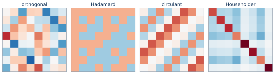
• Lossless means \(\mathbf{A}\) is orthogonal — or diagonally similar to one. is_orthogonal and is_unilossless check it; it is not a matter of faith
• Orthogonal, Hadamard, circulant, Householder — same losslessness, different mixing speed and different cost
• Sparse and structured matrices buy back the \(N \times N\) multiply

Mixing is audible

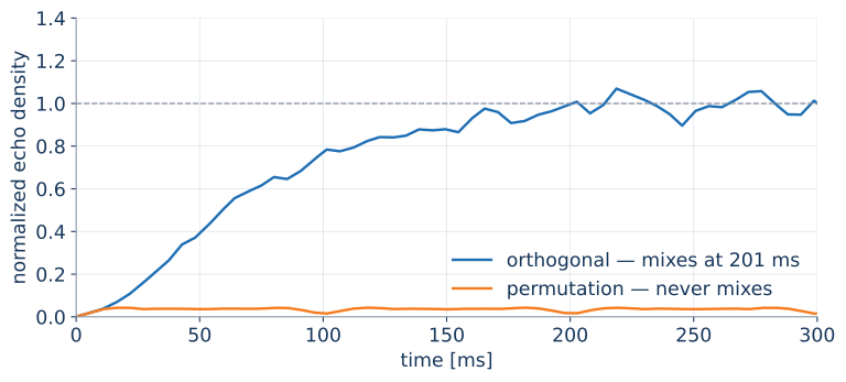
Normalized echo density (Abel & Huang 2006) reaches 1 when the response is statistically Gaussian — that is “mixed”.

• orthogonal: mixes at ~250 ms
• permutation: never mixes — a single long comb filter

Same delays, same decay, same losslessness. Only the matrix changed.

Play both impulse responses. The permutation FDN is the sound of a bad reverb.

Knob 3 — absorption sets the decay

Broadband — attenuate a little on every trip round the loop, proportional to the delay length, so short and long lines die together:

g = pyFDN.rt_to_gain_per_sample(rt, fs)
A_lossy = np.diag(g ** delays) @ A

Frequency-dependent — replace each scalar gain with a filter per delay line whose attenuation follows the target \(T_{60}\) across frequency:

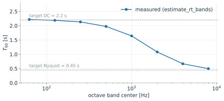
sos = pyFDN.decay_to_geq(target_rt, delays, fs)

Proportional-to-delay is what makes the decay homogeneous, and therefore predictable — a graphic-EQ absorption design preserves that per band.

What decay looks like

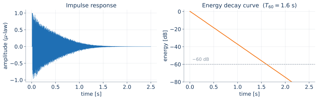
• Impulse response (\(\mu\)-law compressed, so the tail stays visible)
• Energy decay curve = backward energy integral; the \(-60\) dB crossing is \(T_{60}\)

Step 1 — delays

delays = pyFDN.sample_delay_lengths(
    N=8,
    delay_range=(1000, 3000),        # samples ≈ 21–62 ms at 48 kHz
    distribution="geometric",        # or "uniform"
    coprime=True,                    # avoid coinciding echoes
    rng=2,
)
# or set them by hand, in milliseconds:
delays = pyFDN.ms_to_smp(np.array([20, 27, 31, 37, 43, 53, 61, 71]), fs)

Try three delay sets and listen to each:

• short & narrow (300, 600) — flutter, obvious pitch
• long & wide (2000, 9000) — sparse early reflections, granular onset
• coprime vs not — set coprime=False and listen for the ringing

Then look at pyFDN.echo_density(ir, fs=fs) for each.

Step 2 — the matrix

for matrix_type in pyFDN.fdn_matrix_gallery():        # list the options
    A = pyFDN.fdn_matrix_gallery(8, matrix_type)
    print(f"{matrix_type:32s} lossless: {pyFDN.is_unilossless(A)}")

A = pyFDN.fdn_matrix_gallery(8, "orthogonal")

Swap in "permutation", "Householder", "Hadamard" and "orthogonal". For each: listen, then measure the mixing time with pyFDN.echo_density. Which one mixes fastest? Which is cheapest to compute?

The notebook prints the mixing time of an orthogonal and a permutation FDN with the same delays: one mixes in half a second, the other never does.

Step 3 — gains, and your first render

B = np.ones((8, 1)) / np.sqrt(8)      # input  → delay lines
C = np.ones((1, 8)) / np.sqrt(8)      # delay lines → output
D = np.zeros((1, 1))                  # direct path: wet only

ir = pyFDN.dss_to_impz(3 * fs, delays, A, B, C, D).squeeze()

That is a complete FDN — delays, A, B, C, D is the delay state space. With an orthogonal A and nothing in the loop it is lossless, so the tail never decays. Listen to it once; it is the sound of energy with nowhere to go.

Set D = 0.5 to mix the dry signal back in, then drive a single delay line with B = np.eye(8)[:, :1] and listen to how much later the tail fills in.

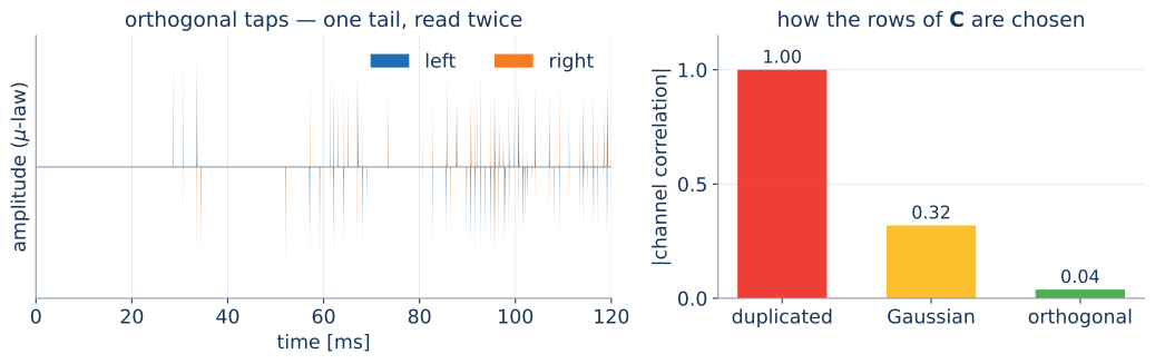
Stereo — one tail, two taps

duplicated

orthogonal

C = pyFDN.random_orthogonal(N)[:2]    # (2, N)
D = np.zeros((2, 1))

Same loop, same decay — only the tap differs. The rows have to be orthogonal, not merely different.

Step 4 — decay you can specify

# broadband: bake a homogeneous gain into the loop
g = pyFDN.rt_to_gain_per_sample(rt=1.8, fs=fs)
A_lossy = np.diag(g ** delays) @ A

# frequency-dependent: one graphic-EQ absorption filter per line, inside the loop
target_rt = np.array([2.4, 2.4, 2.3, 2.1, 1.8, 1.4, 1.0, 0.7, 0.5, 0.5])
absorption = pyFDN.decay_to_geq(target_rt, delays, fs)

build = pyFDN.FDNBuild(A=A, B=B, C=C, D=D, delays=delays, fs=fs, post_delay=absorption)
ir = pyFDN.build_to_impz(build, 3 * fs).squeeze()

Then check that you got what you asked for:

rt_measured, f_center = pyFDN.estimate_rt_bands(ir, fs)
print(np.round(rt_measured, 2))      # ← compare against target_rt[1:9]

Ask for something extreme — 4 s at 63 Hz and 0.2 s at 8 kHz — and see where the design stops delivering. Why does it break?

Step 5 — analyze and listen

pyFDN.plot_FDN_build(build)
pyFDN.plot_impulse_response(ir, fs=fs)
pyFDN.plot_edc(ir, fs=fs)
pyFDN.plot_spectrogram(ir, fs)
pyFDN.echo_density(ir, fs=fs)

dry, _ = pyFDN.load_audio("synth_dry", fs=fs)
wet = pyFDN.process_fdn(
    np.pad(dry, (0, 2 * fs)),             # room for the tail
    delays, A, B, C, D,
    post_delay=td.SOSBank(absorption),    # absorption in the loop
)

Checkpoint. Get an FDN you like the sound of. Then break it: make it metallic on purpose, and say which knob did it.

One more turn — the hooks

process_fdn takes a filter at three points in the loop, and each one is a whole family of reverbs. Any object with a .filter(block) method fits.

wet = pyFDN.process_fdn(
    x, delays, A, B, C, D,
    post_delay=td.SOSBank(absorption),                     # absorption
    post_matrix=td.TimeVaryingMatrix(8, 10.0, 1.1, fs, 0.7),  # a moving matrix
)

Swap post_matrix for td.ControllableFullWaveRect(8, 0.25, [4, 5, 6, 7]) — half the lines partly rectified. The harmonics you hear were never in the input; the FDN is generating them, and there is no transfer function left to plot. Take alpha up toward 1.0 and listen to how far you can push it before it stops sounding like a room.

Same three hooks as the figures in part 1: post_delay, post_matrix, post_output.

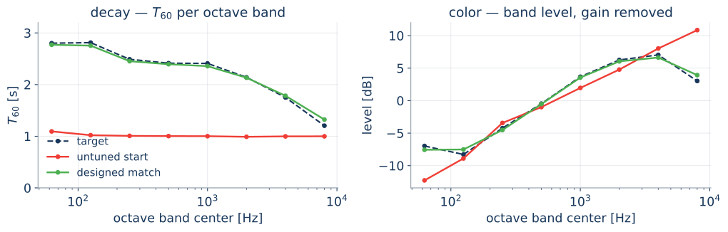
Now match a real room

Pori concert hall — pyFDN.load_audio("s3_r4_o")

Navy the hall, red the notebook as it opens, green a designed match.

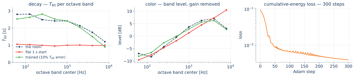
Last section of the notebook: turn the knobs you already have until you get as close as you can. Decay first — the color mostly follows. Mixing time last.

5 · Hands-on 2 — match a room with gradients

Open the second notebook

examples/example_train_fdn_to_rir.py — the same hall you just chased by hand, this time fitted by an optimizer.

1. Open it in molab, Fork, run all cells
2. Two dropdowns at the top decide everything downstream:
   • Run on — CPU, or the GPU if your runtime has one
   • EQ design — a first-order shelf (2 numbers) or a ten-band graphic EQ (10)

Start the run now. The rest of this section is a commentary on what it is doing while it does it.

uv pip install "pyfdn[examples]"
marimo edit examples/example_train_fdn_to_rir.py

300 Adam steps, float32, \(2^{17}\)-point grid:

• ≈ 90 s on a laptop CPU
• pick a CUDA GPU in the dropdown and the model, the loss and the excitation all move with it — the recursion is a batched complex solve over 65 537 bins, which is the shape a GPU likes
• not Apple MPS: that same complex solve is unimplemented there, as is the matrix_exp the orthogonal parametrization needs

Why gradients

What we can do analytically

• delays → modal density
• absorption filters → \(T_{60}(\omega)\)
• unitary matrix → losslessness

These are invertible designs: state the target, get the parameters. That was the last slide of Hands-on 1, and it got you close.

What we cannot

• “make it not sound metallic”
• “match this hall, all of it, at once”
• “stay flat and mix fast and use a sparse matrix”

No closed form. But every one of them is a differentiable loss.

The FDN is a recursive filter with \(N^2 + 2N + 1\) scalars and two filter banks. Write the objective, and let autograd find them.

The plan

One notebook, one target, seven steps — and three of them are the ones that actually decide whether this works:

1. The target, and the yardstick we will not let the fit see
2. The start — a generic 1 s reverberator that knows nothing about the room
3. The parametrization — what has a gradient, and in what units ⚠️
4. The loss — the obvious one is wrong, and there is a table to prove it ⚠️
5. Train — 300 Adam steps, one loss curve
6. Read the answer out — two filters, both plottable
7. Measure — octave-band \(T_{60}\) and level, against numbers the fit never saw

Everything here needs torch, via FLAMO. If the install did not work, the notebook is rendered in full with its plots and audio.

FLAMO in one slide

FLAMO — frequency-domain differentiable audio processing (Dal Santo, De Bortoli, Prawda, Schlecht & Välimäki, ICASSP 2025)

• audio modules as torch.nn.Modules: Delay, Gain, Filter, SVF, …
• composition primitives: Series, Parallel, Recursion, Shell
• the loop is closed in the frequency domain — a Recursion becomes a matrix inverse over FFT bins, so there is no per-sample unrolling and no vanishing-gradient problem over a 3-second tail

model = pyFDN.trainable_from_build(build, nfft=2**17, device=device)  # cpu or cuda
pyFDN.plot_flamo_graph(model)

pyFDN’s job is to hand FLAMO a correct FDN — admissible matrices, homogeneous decay, sane initialization — and to read the result back out.

Step 1 — the target, and the exam paper

Pori concert hall — pyFDN.load_audio("s3_r4_o"), trimmed to the direct sound, normalized to unit energy

est_rt, f_centre = pyFDN.estimate_rt_bands(rir, fs)
est_level, _ = pyFDN.estimate_initial_level_bands(rir, est_rt, fs)
# 2.8 s at 63 Hz → 1.2 s at 8 kHz

In Hands-on 1 these two lines were the design. Here they are the exam paper: computed once, fed to nothing, and compared against at the very end.

That separation is the whole reason the result means anything. A fit scored on the quantity it was optimizing tells you only that the optimizer works.

Step 2 — a reverberator that knows nothing

init_build = pyFDN.fdn_build_gallery(
    delays=pyFDN.sample_delay_lengths(
        16, (700, 2500), distribution="geometric", coprime=True, rng=1
    ),
    fs=fs, io_type="normalized", direct_gain=0.0,
    rt=1.0, rt_nyquist=1.0,        # flat 1 s — the entire prior knowledge of the room
    rng=0,
)

A complete FDN, not a scaffold: random orthogonal matrix, normalized gains, flat 1 s absorption. The room runs 2.8 s to 1.2 s, so this start is wrong by a factor of three at the bottom and by a fifth at the top — and wrong in opposite directions at the two ends, which is the part no single scalar can fix.

The one thing the measurement is allowed to set before the optimizer runs is the overall energy — one scalar on the output gain. Comment it out and watch the first fifty steps get spent on a volume knob.

Step 3 — parametrize by what you would plot

post_delay = pyFDN.DecayFilter(1.0, delays, fs, design=design)
post_output = pyFDN.OutputEQ(0.0, 1, fs, design=design)

what	trained as
decay, post_delay	\(T_{60}\) in seconds
color, post_output	gain in dB
mixing, \(\mathbf{A}\)	on \(SO(N)\)
level, \(\mathbf{B}\,\mathbf{C}\,\mathbf{D}\)	directly
the delays	fixed — integers

Train the attenuation filter’s coefficients and it diverges within fifty steps at any learning rate: a too-quiet FDN offers every loss the same cheap direction — more loop gain.

\[\mathrm{RT}_k \to \underbrace{\tfrac{-60\,d_i}{\mathrm{RT}_k f_s}}_\text{dB per round trip} \to \text{biquads}\]

A positive RT is a contractive loop for every value the parameter can take. The stability constraint is gone, not enforced — and the same trick puts the output EQ in dB.

Step 4 — why not a spectrogram distance

Freeze everything but the decay, scale the room’s measured \(T_{60}\) by a constant, and score it on a mel multi-resolution spectrogram distance:

\(T_{60}\) scale	0.4	0.6	1.0	1.3	1.6
mel MSS (\(\times 10^{-5}\))	1.819	1.804 ← minimum	1.855	1.924	2.009
energy decay at 1 s	−67 dB	−47 dB	−31 dB	−25 dB	−21 dB
the room, at 1 s			−29 dB

An FDN whose tail is 18 dB below the room’s scores better than the one that tracks it to within 2 dB. Not a bug: two rooms with the same decay still have uncorrelated fine structure, and against detail you cannot predict, silence is a better guess than the right amount of the wrong detail.

Step 4 — a loss that can see a decay

loss = pyFDN.MatchCumulativeEnergy(rir, window=1024, power=0.5, frequency="both")

\[E[f, t] \;=\; \sum_{t' \ge t} \; \sum_{f' \ge f} \big| S[f', t'] \big|^2\]

• backwards in time = Schroeder integration — the decay itself
• along frequency = what octave bands do, without band edges: every bin is compared against every wider band containing it

• read the \(t=0\) edge → the integrated spectrum
• read the \(f=0\) edge → the energy decay curve
• one term, no weight to tune — there is nothing to weigh it against

frequency="descending" cumulates high→low only. The bottom octave loses its gradient and the fit abandons it: 63 Hz lands at 0.26 s against the room’s 2.8 s. Run it and look at the trained \(T_{60}\) curve.

Steps 5–7 — train, read out, measure

the room

flat 1 s start

trained

From a flat 1 s decay and a flat EQ: 52 % → 10 % mean \(T_{60}\) error, and 1.71 dB → 0.79 dB of band-level shape. Nothing the estimators report was ever shown to the optimizer.

Two numbers or ten?

The same fit with the design dropdown in each position, everything else identical:

	mean \(T_{60}\) error	level shape	final loss	wall clock
untrained — flat 1 s	52.4 %	1.71 dB	0.0932	—
first-order shelf — 2 numbers, 1 biquad	9.8 %	0.79 dB	0.0039	90 s
ten-band graphic EQ — 10 numbers, 11 biquads	10.6 %	0.71 dB	0.0026	7 min

• Five times the parameters reach a 35 % lower loss — and a worse \(T_{60}\)
• Per band: the graphic EQ halves the error at 4 k and 8 k, then throws it away at 63 Hz (10 % → 30 %), the band the cumulative loss weights least
• The shelf gets that band nearly right by not being free — its low plateau is pinned by the whole midrange
• Extra parameters are only worth what the objective can supervise

The deliverable

trained_build = pyFDN.extract_build(model)      # plain NumPy, no torch

Both trained filters come back baked as ordinary SOS banks in post_delay and post_output. Nothing about the build remembers that an optimizer produced it — so it goes straight into build_to_impz, process_fdn, or the FAUST export from part 2.

Run dry audio through the reverb you just trained. Then reopen example_process_fdn and A/B it against the one you tuned by hand.

A different objective, same machinery

• Same train_fdn, same Trainable, no target signal at all: loss = magnitude flatness (MSE in dB) + a sparsity penalty on \(\mathbf{A}\)
• Trains a lossless FDN, so the decay is added afterwards with build_set_decay — and alias_decay_db becomes mandatory, because poles on the unit circle make the frequency-domain inverse near-singular
• Dal Santo, Prawda, Schlecht & Välimäki, Differentiable FDN for Colorless Reverberation (DAFx 2023)

example_train_colorless_FDN — converges in seconds on a laptop CPU.

Where it goes wrong

• The parametrization matters more than the optimizer. Raw filter coefficients diverge at every learning rate; \(T_{60}\) in seconds converges.
• The loss is not your ear. Cumulative energy sees the decay. It does not see roughness, flutter, or the early pattern.
• The loss decides which parameters are worth having. A band the objective barely weights is a band extra freedom makes worse.
• Overfitting to one RIR gives you a reverb that only works for that room.
• nfft is a resolution knob, not a performance knob — it has to hold the decay you are fitting, and it is structural in FLAMO, so it cannot be changed after the model is built.

Break it on purpose and read the failure off the loss curve, not the audio: max_steps=20, lr=1.0, frequency="descending", loss = pyFDN.MatchMelSpectrogram(rir). Each fails differently.

Thank you, pyFDN contributors

Sebastian J. Schlecht

Facundo Franchino

Jeremy Bai

Alma Hova

Orchisama Das

Bharadwaj Lakuduva Suresh Babu

Cristóbal Andrade

Gloria Dal Santo

Gian Marco De Bortoli

Questions

Tutorial: artificial-audio.github.io/pyfdn-tutorial-2026 · pyFDN docs: artificial-audio.github.io/pyFDN