Estimation Is Projection

Why the best linear estimate is a right angle

Half a face from the other half

\[ % Number sets \newcommand{\Nat}{\mathbb{N}} \newcommand{\Integer}{\mathbb{Z}} \newcommand{\Real}{\mathbb{R}} \newcommand{\Complex}{\mathbb{C}} % Operators \newcommand{\SNR}{\operatorname{SNR}} \newcommand{\tr}{\operatorname{tr}} \newcommand{\re}{\operatorname{Re}} \newcommand{\im}{\operatorname{Im}} \newcommand{\sign}{\operatorname{sign}} \newcommand{\rect}{\operatorname{rect}} \newcommand{\sinc}{\operatorname{si}} \newcommand{\erf}{\operatorname{erf}} \newcommand{\erfc}{\operatorname{erfc}} \newcommand{\kurt}{\operatorname{kurt}} \newcommand{\diag}{\operatorname{diag}} \newcommand{\MSE}{\operatorname{MSE}} \newcommand{\argmin}{\operatorname*{argmin}} \newcommand{\argmax}{\operatorname*{argmax}} \newcommand{\bias}{\operatorname{bias}} \newcommand{\Bin}{\operatorname{Bin}} % Delimiters \newcommand{\paren}[1]{\left(#1\right)} \newcommand{\bracket}[1]{\left[#1\right]} \newcommand{\set}[1]{\left\{#1\right\}} \newcommand{\abs}[1]{\left\lvert #1 \right\rvert} \newcommand{\norm}[1]{\left\lVert #1 \right\rVert} \newcommand{\ip}[1]{\left\langle #1 \right\rangle} % Notation \newcommand{\dd}{\,\mathrm{d}} \newcommand{\tran}{^{\top}} \newcommand{\conv}{\ast} \newcommand{\conj}{^{*}} \newcommand{\herm}{^{\mathsf{H}}} \newcommand{\opt}{^{\star}} % Expectation and variance % \newcommand{\E}[1]{\mathbb{E}\!\left[#1\right]} \newcommand{\E}[2][]{\mathbb{E}_{#1}\!\left[#2\right]} \newcommand{\Var}[1]{\mathbb{V}\!\left[#1\right]} % Distributions \newcommand{\Gauss}{\mathcal{N}} \newcommand{\Uniform}{\mathcal{U}} \newcommand{\FT}{\mathcal{F}} % Probability \newcommand{\Prob}[1]{\mathbb{P}\!\left(#1\right)} % Misc \newcommand{\bsy}[1]{\boldsymbol{#1}} \newcommand{\calR}{\mathcal{R}} \newcommand{\calC}{\mathcal{C}} \]

Guessing what you cannot see

Three portraits the estimator never saw. Left to right: the observed left half, the estimate written into the right half, the truth, the error. Far right: the error the estimator predicts for each pixel, before seeing any face.

The estimate is a linear combination of the 2048 visible pixels, and it needs nothing but the covariance matrix of the random-vector week. This week shows why that combination is found by drawing a right angle.

This is the pivot of the course. Everything after it is this week’s projection with a different set of observations.

The plan for the week

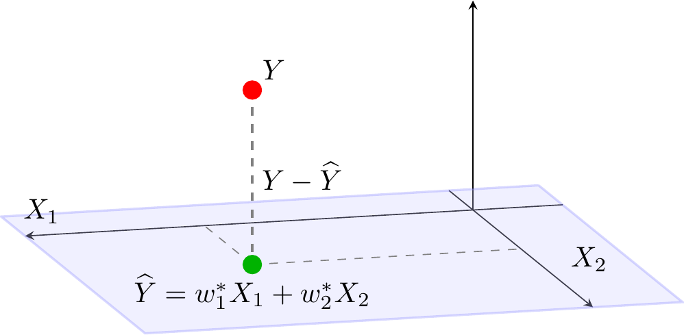
The principle. Random variables are vectors, the mean-square error is a squared distance, and the best estimate is a perpendicular dropped onto the observations: the normal equations.

Four readings of the same equation. A richer list of observations; the Gaussian case, where linear is already optimal; data instead of moments (least squares); and observations that arrive one at a time (innovations).

In the notes Random Variables as Vectors · The Orthogonality Principle and Normal Equations · Linear and Affine MMSE Estimation · Vector Targets and the Error Covariance · Beyond the Affine Estimator · Gaussian Estimation · Least Squares · Sequential Estimation and the Innovations

Random variables are vectors

A random variable is a list

A random variable is a map from outcomes to numbers. On a finite sample space \(H=\set{\eta_1,\dots,\eta_M}\) it is nothing but the list of its values: \[X\;\longleftrightarrow\;\big[X(\eta_1),\ X(\eta_2),\ \dots,\ X(\eta_M)\big]\in\Complex^M .\]

One coordinate per outcome: not per sensor, not per time index. A linear combination \(aX+bY\) is the coordinatewise combination, and all of vector geometry applies.

…with the coordinates weighted by probability

Outcomes have different probabilities, so the inner product weights each coordinate: \[\sum_mX(\eta_m)\,Y\conj(\eta_m)\,\Prob{\eta_m}=\E{XY\conj}.\]

Inner product of random variables \[\ip{X,Y}=\E{X\,Y\conj},\qquad\norm{X}^2=\E{\abs X^2}.\]

Expectation is the inner product. The probability measure says how much each coordinate counts, and the conjugate makes \(\norm X^2\) a real, nonnegative power.

The dictionary

vectors	random variables
inner product \(\mathbf y\herm\mathbf x\)	correlation \(\E{XY\conj}\)
squared length	power \(\E{\abs X^2}\)
orthogonal	uncorrelated (zero mean)
cosine of the angle	correlation coefficient \(\rho\)
Gram matrix	correlation matrix \(\mathbf R_{\mathbf{XX}}\)
squared distance \(\norm{\mathbf y-\widehat{\mathbf y}}^2\)	mean-square error \(\E{\abs{Y-\widehat Y}^2}\)
orthogonal projection	the optimal linear estimator

Read the last two rows together and the whole week is already visible.

Two consequences, for free

Inherited from the geometry

• Cauchy–Schwarz, \(\abs{\ip{X,Y}}\le\norm X\norm Y\): a correlation coefficient is a cosine.
• Pythagoras, \(X\perp Y\Rightarrow\norm{X+Y}^2=\norm X^2+\norm Y^2\): powers of uncorrelated signals add.

Pythagoras is the workhorse. Every optimality proof below that says “the error is orthogonal, therefore nothing shorter exists” is that one line.

The principle

The problem

Estimate a zero-mean target \(Y\) from observations \(\mathbf X=[X_1,\dots,X_N]\tran\) by a linear combination, and choose the weights to minimize the mean-square error: \[\widehat Y=\mathbf w\herm\mathbf X=\sum_kw_k\conj X_k,\qquad J(\mathbf w)=\E{\abs{Y-\widehat Y}^2}=\norm{Y-\widehat Y}^2 .\]

The linear MMSE estimator as a block diagram: observations weighted and summed, the error minimized.

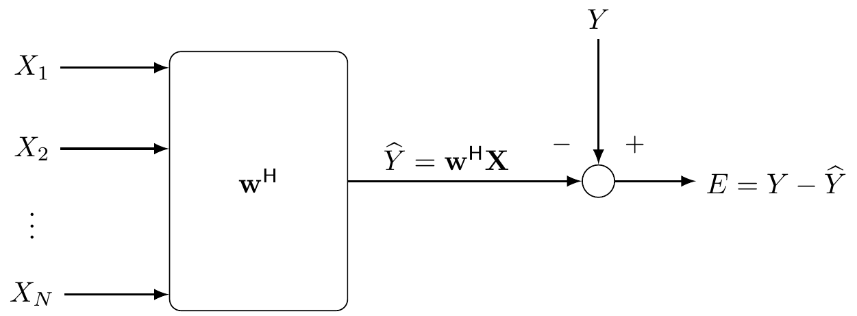
In the dictionary: find the point of \(\mathrm{span}\set{X_1,\dots,X_N}\) closest to \(Y\). That is a projection, and projections are characterized by a right angle.

The orthogonality principle

Orthogonality principle \(\widehat Y\) minimizes \(\E{\abs{Y-\widehat Y}^2}\) if and only if the error is orthogonal to every observation: \[\E{(Y-\widehat Y)\,X_k\conj}=0,\qquad k=1,\dots,N.\]

The orthogonality principle

The target \(Y\), the plane spanned by the observations, and the error standing perpendicular to it.

“Minimize the mean-square error” and “drop a perpendicular” are the same instruction.

Why it is true

Let \(\widetilde Y\) be any competitor in the span. Split its error: \[Y-\widetilde Y=\underbrace{(Y-\widehat Y)}_{\perp\text{ the span}}+\underbrace{(\widehat Y-\widetilde Y)}_{\in\text{ the span}} \quad\Longrightarrow\quad \norm{Y-\widetilde Y}^2=\norm{Y-\widehat Y}^2+\norm{\widehat Y-\widetilde Y}^2\ge\norm{Y-\widehat Y}^2 .\]

Equality only when \(\widetilde Y=\widehat Y\): optimal and unique.

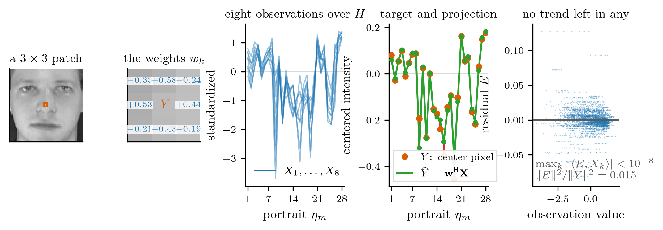
The converse is the one used in practice: any correlation left between the error and an observation is information not yet used.

If \(\varepsilon_k=\E{(Y-\widehat Y)X_k\conj}\neq0\), nudging the estimate along \(X_k\) lowers the error by \(\abs{\varepsilon_k}^2/\E{\abs{X_k}^2}\).

The normal equations

Substitute \(\widehat Y=\mathbf w\herm\mathbf X\) into the orthogonality conditions:

Normal equations \[\mathbf R_{\mathbf{XX}}\,\mathbf w=\mathbf r_{\mathbf{XY}},\qquad \mathbf R_{\mathbf{XX}}=\E{\mathbf X\mathbf X\herm},\quad \mathbf r_{\mathbf{XY}}=\E{\mathbf X\,Y\conj},\] \[\mathbf w\opt=\mathbf R_{\mathbf{XX}}^{-1}\mathbf r_{\mathbf{XY}},\qquad J_{\min}=\sigma_Y^2-\mathbf r_{\mathbf{XY}}\herm\mathbf R_{\mathbf{XX}}^{-1}\mathbf r_{\mathbf{XY}} .\]

Transposed, the same condition is the equation for the map: \(\mathbf w\herm\mathbf R_{\mathbf{XX}}=\mathbf r_{\mathbf{YX}}\), with \(\mathbf r_{\mathbf{YX}}=\E{Y\mathbf X\herm}=\mathbf r_{\mathbf{XY}}\herm\).

One rule names every correlation: \(R_{XY}=\E{XY\conj}\), first index plain, second conjugated. Swapping the subscripts is taking the adjoint.

The same equations by differentiation

\(J(\mathbf w)=\sigma_Y^2-\mathbf w\herm\mathbf r_{\mathbf{XY}}-\mathbf r_{\mathbf{XY}}\herm\mathbf w+\mathbf w\herm\mathbf R_{\mathbf{XX}}\mathbf w\) is a real quadratic in complex weights. Treating \(\mathbf w\) and \(\mathbf w\conj\) as independent (Wirtinger calculus), \[\frac{\partial J}{\partial\mathbf w\conj}=\mathbf R_{\mathbf{XX}}\mathbf w-\mathbf r_{\mathbf{XY}}=\mathbf 0 .\]

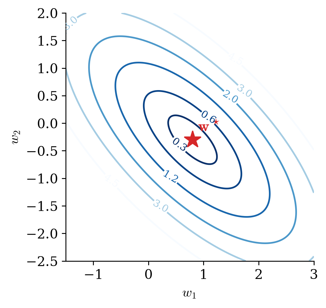
Completing the square shows it is a bowl with its bottom at \(\mathbf w\opt\): \[J(\mathbf w)=J_{\min}+(\mathbf w-\mathbf w\opt)\herm\mathbf R_{\mathbf{XX}}(\mathbf w-\mathbf w\opt).\]

Calculus and geometry give the same answer, as they must. The geometry says why; the calculus is what you run when the cost is not a distance.

The error surface

Figure 1: Contours of J(w) for two weights: ellipses shaped by the eigenvectors and eigenvalues of R_XX, centered on the optimum.

Correlated observations tilt and stretch the bowl. The more elongated it is (the larger the eigenvalue spread), the flatter its floor along one direction, and the less well the data pin that direction down.

How to read the solution

\[\mathbf w\opt=\underbrace{\mathbf R_{\mathbf{XX}}^{-1}}_{\text{correct for overlap}}\ \underbrace{\mathbf r_{\mathbf{XY}}}_{\text{raw similarity}}\]

The raw similarities \(\E{X_kY\conj}\) overcount whatever the observations share with each other. \(\mathbf R_{\mathbf{XX}}^{-1}\) removes the double-counting. If the observations are orthonormal, \(\mathbf R_{\mathbf{XX}}=\mathbf I\) and the weights are just the similarities.

And \(J_{\min}\) is Pythagoras again: the target’s squared length minus the squared length of its shadow. The error never exceeds \(\sigma_Y^2\) (answering \(0\)), and an extra observation can only lower it.

What ignoring the overlap costs

Figure 2: Two sensors X_k = Y + N_k of a unit-power target, noise power 1, with noise correlation ρ between the sensors: the error of the normal-equation weights, and of weights computed as if the noises were uncorrelated.

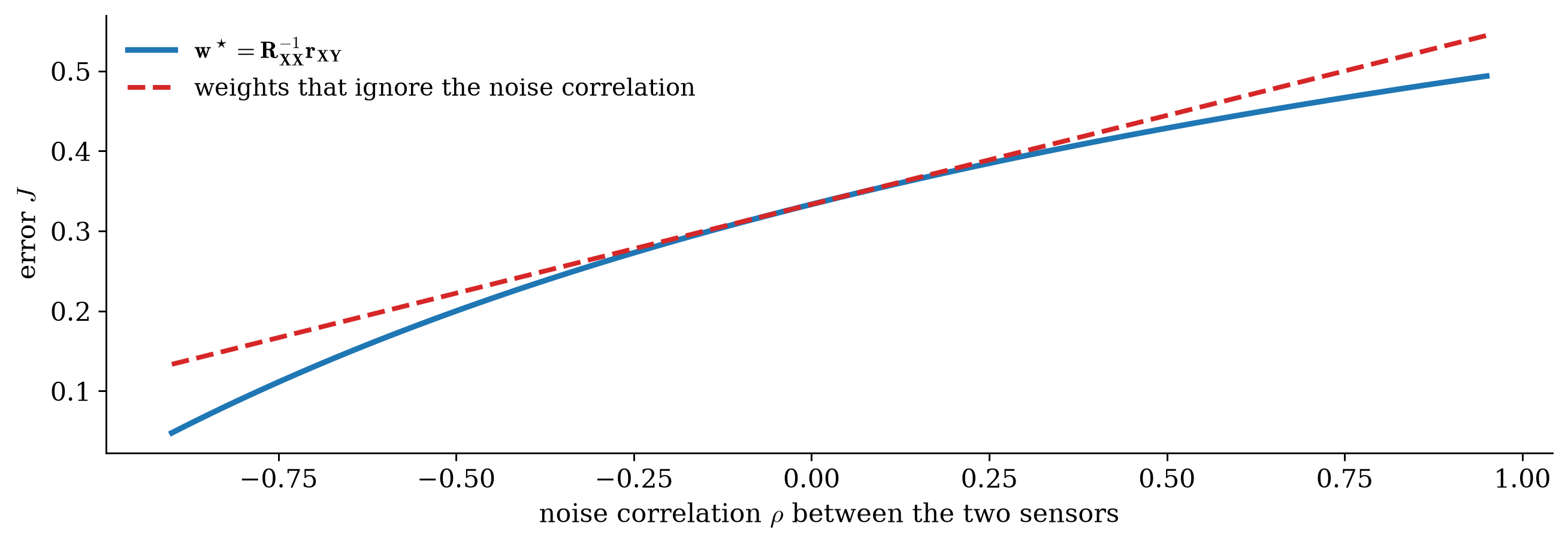
With correlated noise the two readings repeat each other’s errors, and the raw similarities overcount them. \(\mathbf R_{\mathbf{XX}}^{-1}\) corrects for it; with anticorrelated noise it even exploits the cancellation.

A four-outcome example

Four equally likely outcomes, so a random variable is a list of four numbers: \[X_1=[1,1,-1,-1],\qquad X_2=[1,-1,1,-1],\qquad Y=[3,1,1,-1].\]

Figure 3: The observations, the target, its projection and the residual, one bar per outcome.

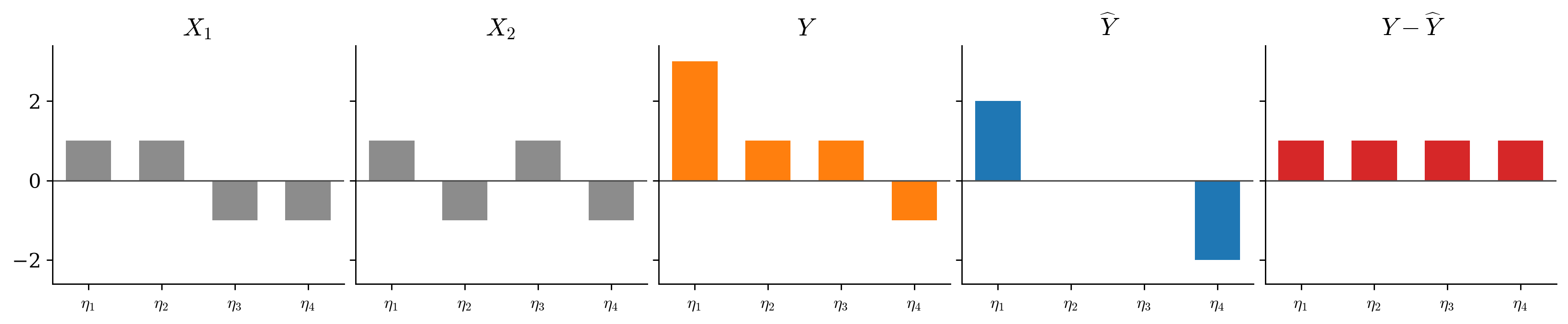
\(\ip{X_1,X_2}=0\), so \(\mathbf R_{\mathbf{XX}}=\mathbf I\) and \(w_1=\ip{Y,X_1}=1\), \(w_2=\ip{Y,X_2}=1\). The residual \([1,1,1,1]\) is constant: the mean of \(Y\), which no zero-mean combination can reach.

With nonzero means: the affine estimator

Estimate the fluctuation and add the mean back:

Affine MMSE estimator \[\widehat Y=m_Y+\mathbf c_{\mathbf{XY}}\herm\mathbf C_{\mathbf{XX}}^{-1}(\mathbf X-\mathbf m_{\mathbf X}),\qquad \mathbf c_{\mathbf{XY}}=\E{(\mathbf X-\mathbf m_{\mathbf X})(Y-m_Y)\conj}.\]

Same equations, covariances in place of correlations. With no data the estimate is \(m_Y\) and the error \(\sigma_Y^2\); every observation is a correction to the prior mean.

The whole estimator needs four moments, \(\mathbf m_{\mathbf X}\), \(m_Y\), \(\mathbf C_{\mathbf{XX}}\), \(\mathbf c_{\mathbf{XY}}\), and one matrix solve.

Two noisy sensors, once more

Two readings \(X_k=Y+N_k\) Target power \(\sigma_Y^2\), independent noise \(\sigma_1^2,\sigma_2^2\). Then \(\mathbf R_{\mathbf{XX}}=\sigma_Y^2\mathbf 1\mathbf 1\tran+\diag(\sigma_1^2,\sigma_2^2)\) and \(\mathbf r_{\mathbf{XY}}=\sigma_Y^2\mathbf 1\), and the normal equations give \[\widehat Y=\frac{x_1/\sigma_1^2+x_2/\sigma_2^2}{1/\sigma_Y^2+1/\sigma_1^2+1/\sigma_2^2},\qquad \frac{1}{J_{\min}}=\frac{1}{\sigma_Y^2}+\frac{1}{\sigma_1^2}+\frac{1}{\sigma_2^2}.\]

The precision-weighted fusion of the Bayesian week, with the prior as a third sensor reading \(0\), recovered from second moments alone and without assuming Gaussian noise.

With numbers: one pixel from its eight neighbors

Left: a \(3\times3\) patch of the portraits and the weights the normal equations give its border pixels. Middle: observations, target, projection and residual as shapes over the sample space. Right: the residual is uncorrelated with every observation.

The edge neighbors get about \(+0.5\) each, the corners about \(-0.25\); together they sum to one, an interpolation stencil read off \(\mathbf R_{\mathbf{XX}}\) and \(\mathbf r_{\mathbf{XY}}\) alone, leaving 1.5% of the pixel’s variance.

A vector target: the error covariance

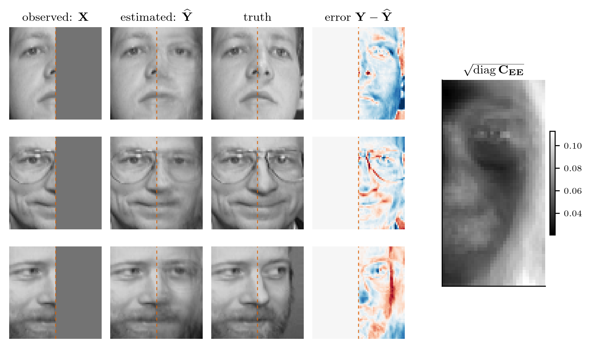
Estimate many targets at once, \(\mathbf Y\) (the whole right half of a face): each component gets its own normal equations, and the errors collect into one matrix:

Error covariance \[\mathbf C_{\mathbf{EE}}=\mathbf C_{\mathbf{YY}}-\mathbf C_{\mathbf{XY}}\herm\mathbf C_{\mathbf{XX}}^{-1}\mathbf C_{\mathbf{XY}} .\] The prior spread, less what the observations explain; its diagonal is the per-pixel error map of the opening slide.

\(\mathbf C_{\mathbf{EE}}\) does not depend on the observed values: how well you will do is known before the measurement arrives. That is what makes it possible to design an experiment.

→ Demo: many sensors, one hidden signal

Correlated sensors are worth less

Figure 4: Normalized error J_min/σ_Y² of the linear MMSE estimate from N sensors, X_k = Y + N_k, with the noises independent or sharing a common component (correlation 0.3).

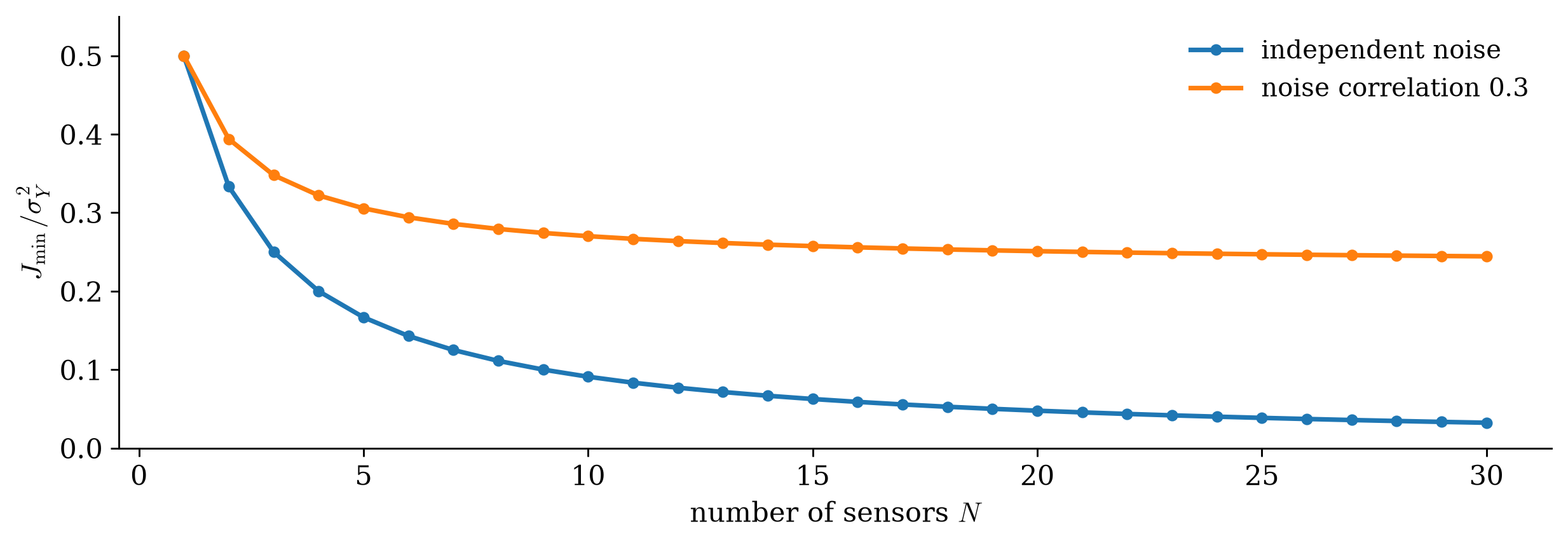
With independent noise the error keeps falling like \(1/N\). With a shared noise component it hits a floor: the common part is the same in every sensor, and no weighting can average it away.

In the eigenbasis

Change the basis, keep the estimate

Any invertible \(\mathbf T\) gives observations \(\mathbf Z=\mathbf T\mathbf X\) with the same span, so the same projection: the weights change, never the estimate or the error.

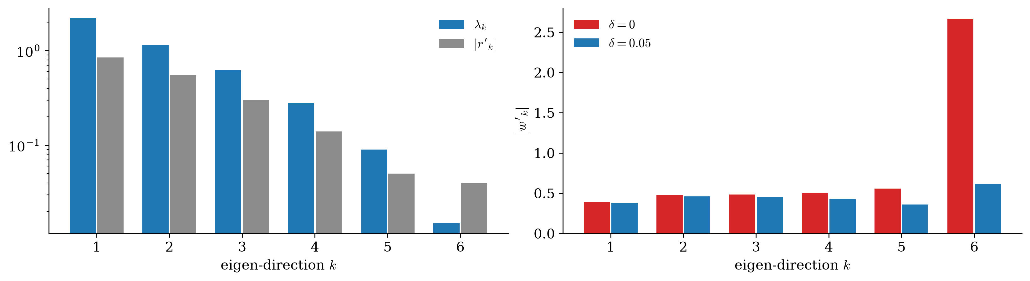
Choose \(\mathbf T=\mathbf U\herm\) from \(\mathbf R_{\mathbf{XX}}=\mathbf U\boldsymbol\Lambda\mathbf U\herm\). Then \(\mathbf R_{\mathbf{ZZ}}=\boldsymbol\Lambda\) and the normal equations fall apart into scalars:

In the eigenbasis \[w'_k=\frac{r'_{k}}{\lambda_k},\qquad J_{\min}=\sigma_Y^2-\sum_k\frac{\abs{r'_{k}}^2}{\lambda_k}.\]

One \(N\times N\) solve becomes \(N\) scalar problems: whiten first, then estimate coordinate by coordinate.

Where it goes wrong

Figure 5: Left: the strength of each eigen-direction and its overlap with the target. Right: the resulting weights, without and with ridge regularization.

Direction 6 holds half a percent of the data’s energy and barely overlaps the target, yet without regularization it gets the largest weight: the estimator amplifies whatever noise lies along it.

Ridge: lift the small eigenvalues

Solve \((\mathbf R_{\mathbf{XX}}+\delta\mathbf I)\mathbf w=\mathbf r_{\mathbf{XY}}\) instead. The eigenvectors stay; every eigenvalue is lifted by \(\delta\):

Ridge \[\widetilde w'_k=\frac{r'_k}{\lambda_k+\delta}=w'_k\cdot\frac{\lambda_k}{\lambda_k+\delta}:\] strong directions untouched, weak ones switched off rather than inverted.

With the moments known, ridge is strictly worse. It earns its place when they are estimated: dividing by a small \(\lambda_k\) amplifies the error in measuring \(r'_k\).

The eigenvalue spread \(\lambda_{\max}/\lambda_{\min}\) says how badly the solve is conditioned, and it is a property of the data, not of the algorithm.

A richer list of observations

Nested subspaces

Two projections The affine functions of the data sit inside all functions of the data. The affine estimator is the projection of \(Y\) onto the first, the conditional mean \(\E{Y\mid\mathbf X}\) the projection onto the second; so \[\E{\abs{Y-\E{Y\mid\mathbf X}}^2}\le\E{\abs{Y-\widehat Y_{\text{aff}}}^2},\] with equality exactly when \(\E{Y\mid\mathbf X}\) is itself affine.

Both are the same question on two admissible sets. The larger set needs the whole joint law; the smaller one needs four moments. The gap between them is the price of computability.

Linear in the weights, not in the data

Project onto any functions \(\psi_k(\mathbf X)\) of the data, a dictionary: the normal equations do not change, only the entries of the Gram matrix.

A projectile’s height against the time of the reading. Left: the best affine estimate is flat. Middle: one more dictionary entry, \(t^2\), recovers the arch. Right: the error against the number of entries.

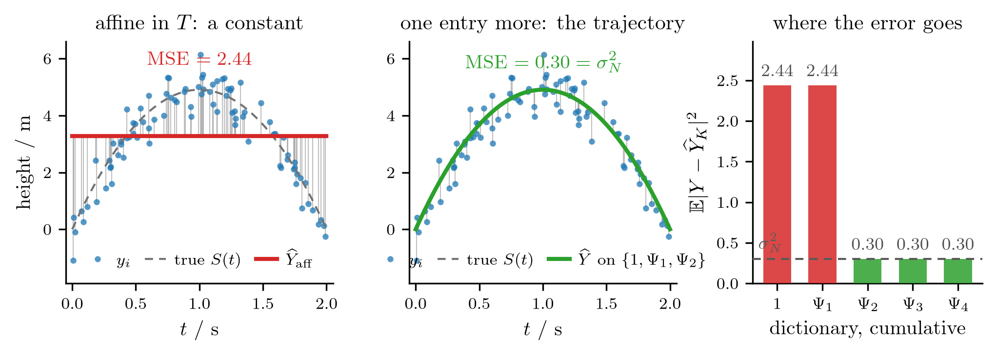
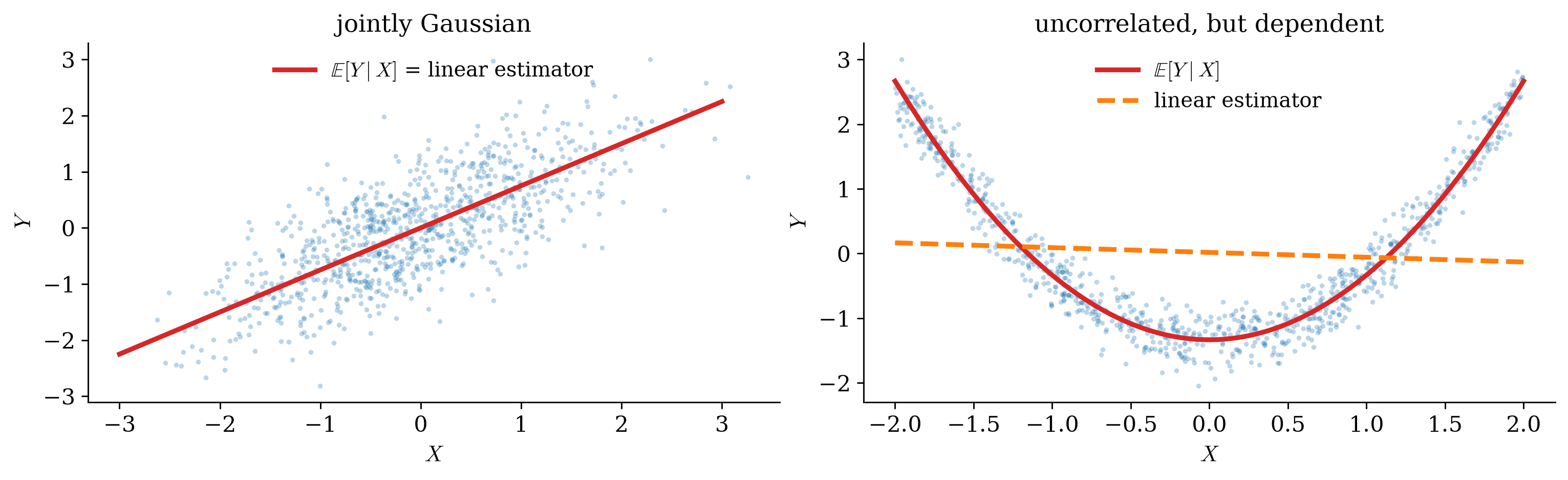
A symmetric arch has no linear part, so the affine estimator sees nothing. Enrich the dictionary and the projection climbs toward the conditional mean; with a complete dictionary it reaches it.

When linear is already optimal

The Gaussian theorem

Gaussian estimation If \((Y,\mathbf X)\) are jointly Gaussian, the conditional mean is affine, \[\E{Y\mid\mathbf X}=m_Y+\mathbf c_{\mathbf{XY}}\herm\mathbf C_{\mathbf{XX}}^{-1}(\mathbf X-\mathbf m_{\mathbf X}),\] so the affine estimator is the best estimator of any kind.

Jointly Gaussian pairs at two correlations: the conditional mean is a straight line, the band one conditional standard deviation \(\sigma_Y\sqrt{1-\rho^2}\).

The proof is three lines, and one of them matters

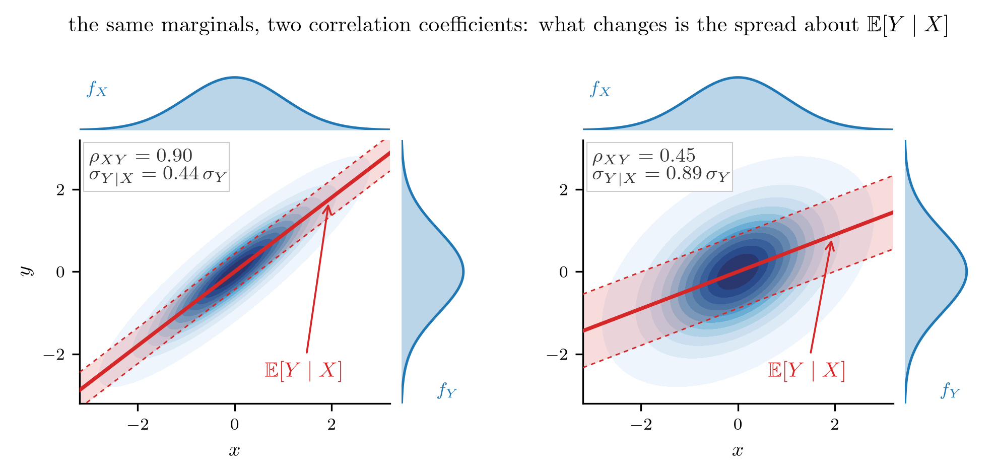
Proof Let \(E=Y-\widehat Y\) be the error of the affine estimator.

1. \(E\) is affine in \((Y,\mathbf X)\), so \((E,\mathbf X)\) is jointly Gaussian.

2. Orthogonality makes \(E\) uncorrelated with \(\mathbf X\), and \(\E{E}=0\).

3. For jointly Gaussian variables, uncorrelated implies independent.

So \(\E{E\mid\mathbf X}=\E{E}=0\), and \(\E{Y\mid\mathbf X}=\widehat Y+\E{E\mid\mathbf X}=\widehat Y\).

Step 3 is the only one that uses Gaussianity. Without it the error is still uncorrelated with the data, but uncorrelated no longer means unpredictable.

What step 3 buys

Figure 6: Left: jointly Gaussian, where the conditional mean is the line the linear estimator finds. Right: uncorrelated but dependent, where the linear estimator sees nothing.

This is why second-order theory carries signal processing: Gaussian noise makes the linear answer the right answer. And where the data are not Gaussian, the covariance can miss everything.

From data instead of moments

Nobody hands you an expectation

\(\mathbf R_{\mathbf{XX}}\) and \(\mathbf r_{\mathbf{XY}}\) are never known. What we hold is \(L\) training pairs \((\mathbf x_i,y_i)\). Two problems, two averages:

Population and empirical risk \[\text{MMSE: }\ \min_{\mathbf w}\ \E{\abs{Y-\mathbf w\herm\mathbf X}^2},\qquad \text{least squares: }\ \min_{\mathbf w}\ \frac1L\sum_{i=1}^L\abs{y_i-\mathbf w\herm\mathbf x_i}^2 .\]

The objectives differ only in which average. So do their solutions.

One substitution

Least-squares normal equations \[\widehat{\mathbf R}_{\mathbf{XX}}\,\mathbf w=\widehat{\mathbf r}_{\mathbf{XY}},\qquad \widehat{\mathbf R}_{\mathbf{XX}}=\frac1L\sum_i\mathbf x_i\mathbf x_i\herm=\frac{\mathbf A\herm\mathbf A}{L},\qquad \widehat{\mathbf r}_{\mathbf{XY}}=\frac1L\sum_i\mathbf x_iy_i\conj ,\] with the design matrix \(\mathbf A\) holding one training input \(\mathbf x_i\herm\) per row.

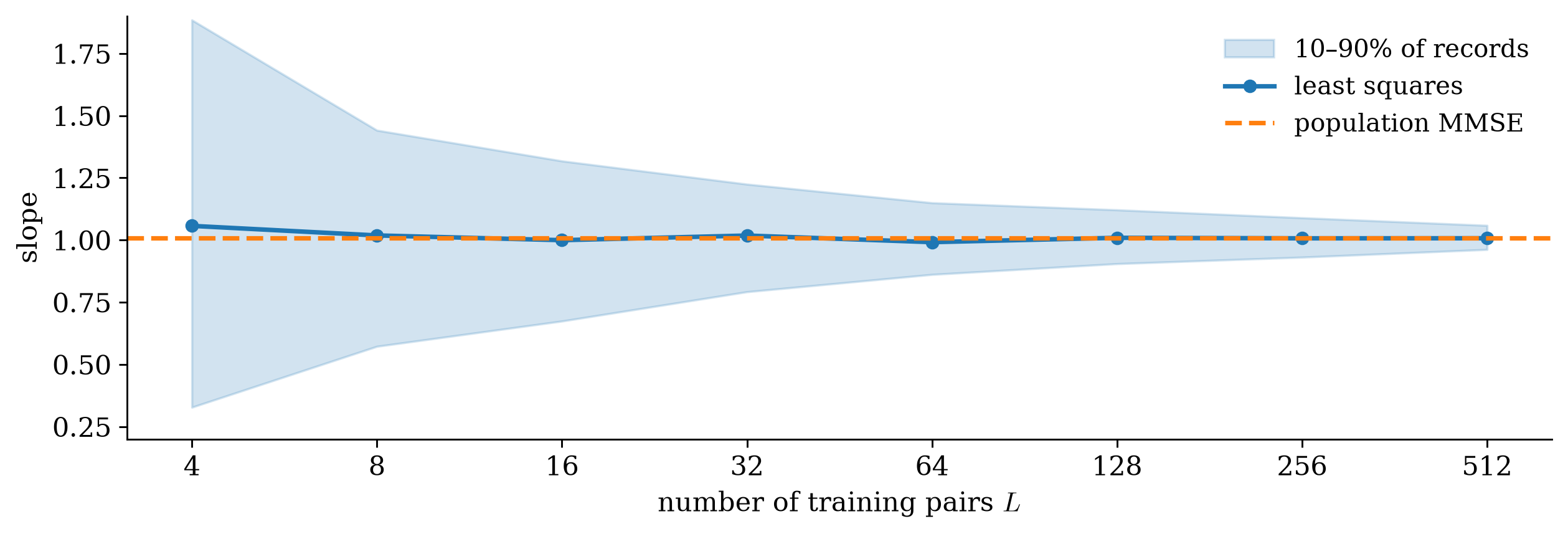
By the law of large numbers the sample moments converge, so the two estimators meet as \(L\to\infty\).

Least squares is MMSE computed with sample moments. There is no second theory, only a second source for the same two objects.

Watching them meet

Figure 7: Least-squares slope over 400 independent records at each sample size, against the population MMSE slope.

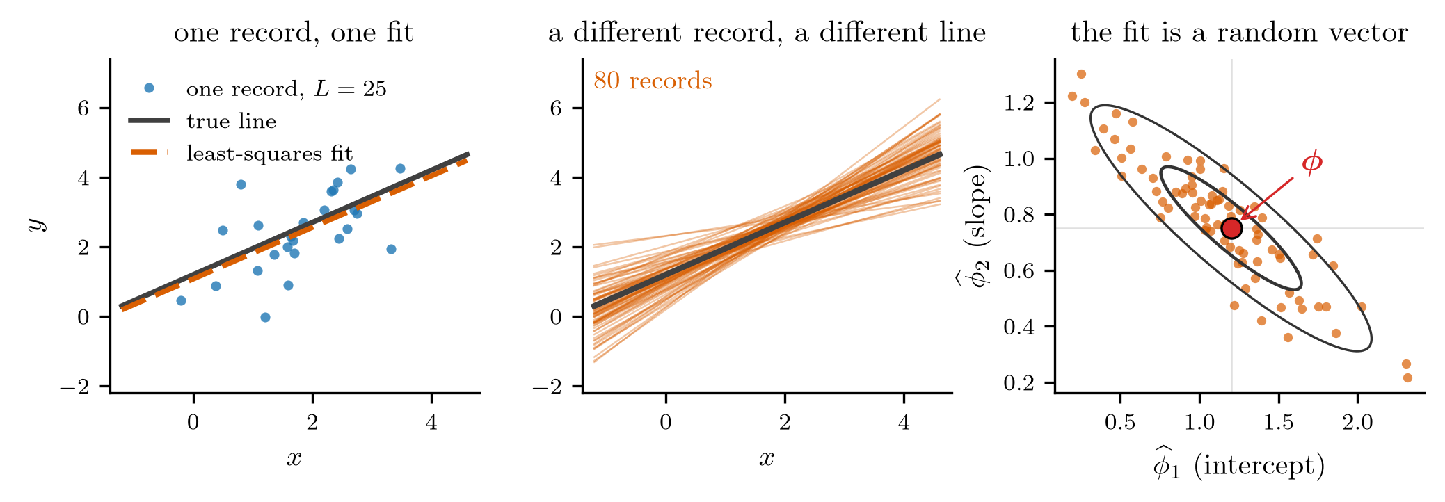
Centered on the right answer from the start; what shrinks with \(L\) is the spread. At small \(L\) the error is in the moments themselves, which is where ridge becomes a necessity.

→ Demo: least squares to MMSE

A fit is an estimator

One record of 25 points and its fitted line; fits from 80 independent records; the two fitted coefficients as a random vector with its covariance ellipse.

The fitted coefficients are a random vector, centered on the truth here, with a covariance ellipse of their own: the error bars of a curve fit.

→ Demo: linear MMSE regression on real data, with ridge

When the data obey a model, the fit is the system

Suppose the outputs really are a matrix applied to the inputs, plus noise uncorrelated with them: \[\mathbf Y=\mathbf A_0\mathbf X+\mathbf N\quad\Longrightarrow\quad \mathbf R_{\mathbf{YX}}=\mathbf A_0\mathbf R_{\mathbf{XX}} .\]

System identification The normal equations \(\mathbf A\,\mathbf R_{\mathbf{XX}}=\mathbf R_{\mathbf{YX}}\) return \(\mathbf A=\mathbf A_0\): the best linear estimator of the output from the input is the system.

From \(K\) pairs, \(\widehat{\mathbf A}=\widehat{\mathbf R}_{\mathbf{YX}}\widehat{\mathbf R}_{\mathbf{XX}}^{-1}\), each row with error covariance \((\sigma_N^2/K)\,\widehat{\mathbf R}_{\mathbf{XX}}^{-1}\): the inputs you choose decide what you learn.

Calibrating a force/torque sensor

Six strain gauges read a six-component load \(\mathbf X=[F_x,F_y,F_z,T_x,T_y,T_z]\tran\) through a \(6\times6\) matrix: \(\mathbf Y=\mathbf A_0\mathbf X+\mathbf N\). Every gauge feels a little of every load.

One forward model, two questions: calibrate (known loads, the matrix sought) and measure (the matrix known, the load sought).

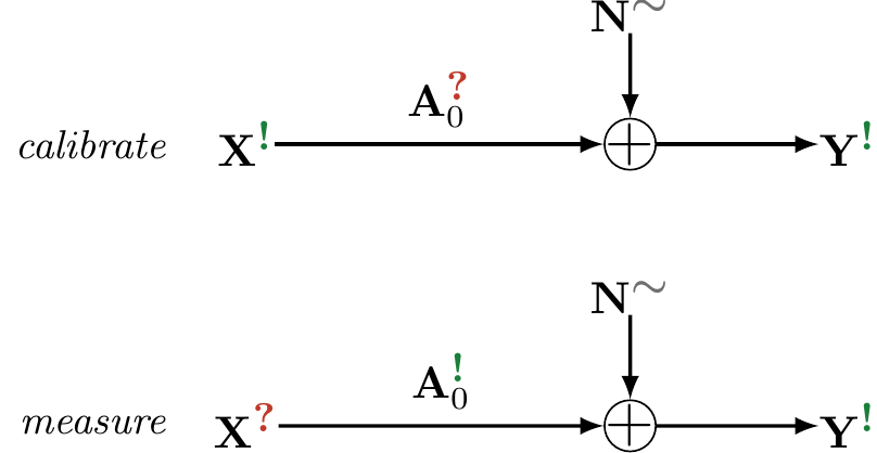
Hang \(K\) known weights, record the readings, solve \(\widehat{\mathbf A}=\big(\sum_k\mathbf y_k\mathbf x_k\tran\big)\big(\sum_k\mathbf x_k\mathbf x_k\tran\big)^{-1}\). Loads \(\pm L\) along each axis, \(m\) times each: every entry has error variance \(\sigma_N^2/(2mL^2)\).

Never twist about \(z\) and the last column of \(\mathbf A_0\) stays unknown, however many weights you hang.

Afterwards the sensor runs backwards, \(\widehat{\mathbf X}=\widehat{\mathbf A}^{-1}\mathbf y\): same model, the question mark moved from the arrow to the input.

Where the right angle lives

Figure 8: The same fit twice. Left: N points in feature space. Right: two vectors in the N-dimensional observation space, where the fit is a right angle.

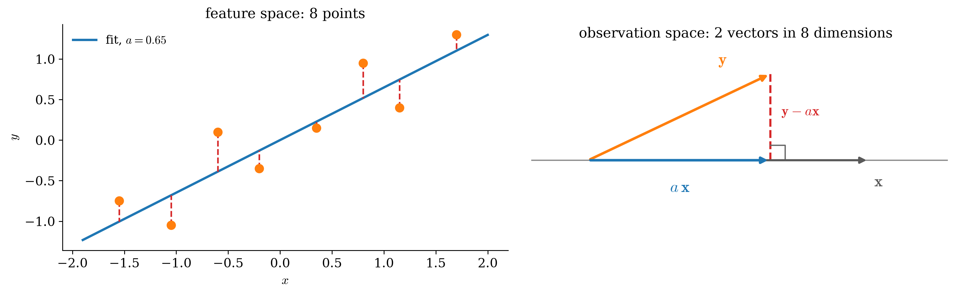
The dashed residuals on the left are the coordinates of one residual vector on the right, and it is perpendicular to \(\mathbf x\). A scatter plot is not the space the projection happens in.

The same right angle in two spaces

space	a vector is	the inner product	the projection is
feature space	one data point	(a drawing only)	nothing
observation space \(\Real^L\)	one variable, sampled \(L\) times	\(\sum_iu_iv_i\conj\)	least squares
random variables	one random variable	\(\E{UV\conj}\)	linear MMSE

The second is the finite-sample approximation of the third: the same right angle, indexed by data point instead of by outcome.

A word on the name

This construction is classically called linear regression, which is unhelpful twice over.

Galton, 1886 Tall parents have less tall children: “regression toward mediocrity”, a statement about one conditional mean, the slope \(\rho\,\sigma_Y/\sigma_X<\sigma_Y/\sigma_X\), not a method of fitting.

What is actually done is to minimize an average squared error: say so.

One observation at a time

The innovation

Take the observations in order.

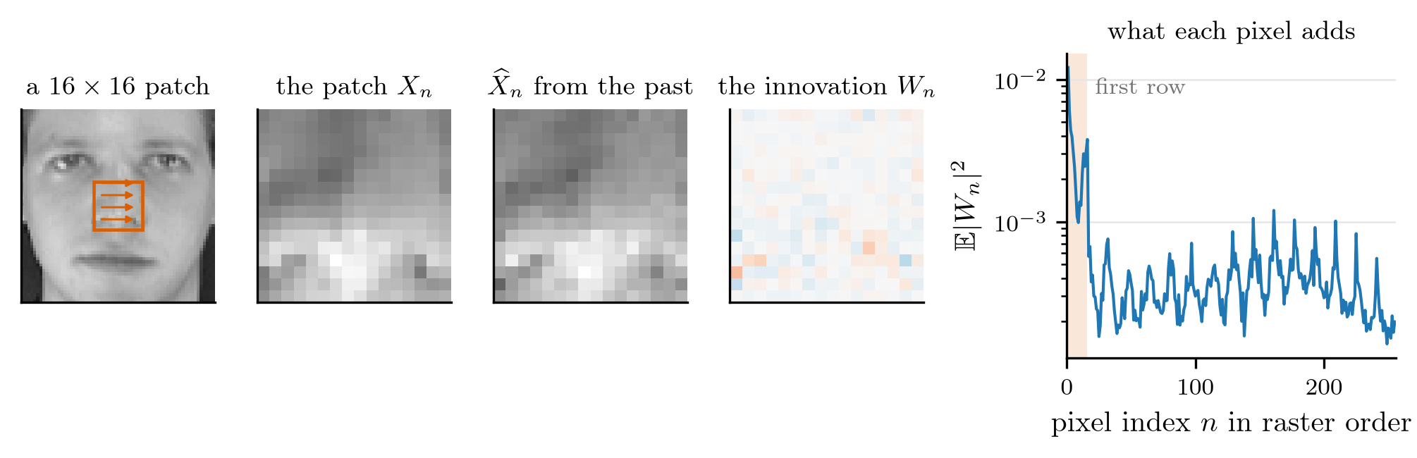
Innovation The part of \(X_i\) its predecessors could not predict linearly: \[W_i=X_i-\widehat X_i,\qquad\widehat X_i=\text{projection of }X_i\text{ onto }\mathrm{span}\set{X_1,\dots,X_{i-1}},\qquad W_1=X_1 .\]

By construction \(W_i\perp X_j\) for every \(j<i\), and each earlier \(W_j\) is a combination of those \(X_j\). So the innovations are mutually uncorrelated, and they span the same space as the observations.

Running the definition along the vector whitens it, one entry at a time.

Innovations are Cholesky

\(W_i\) is \(X_i\) minus a combination of earlier entries, so the map \(\mathbf X\mapsto\mathbf W\) is lower triangular with unit diagonal:

Innovations are the Cholesky factorization \[\mathbf W=\mathbf L^{-1}\mathbf X,\qquad \mathbf R_{\mathbf{XX}}=\mathbf L\mathbf D\mathbf L\herm,\qquad \mathbf D=\diag\paren{\E{\abs{W_i}^2}} .\]

\(\mathbf D^{-1/2}\mathbf L^{-1}\) is the Cholesky whitener of the random-vector week: computing the factor and running all the predictors are the same act.

“Past” was only an ordering. Nothing assumed the index means time: the construction applies to any ordered set of variables with known correlations.

What one more observation buys

Append \(X_{N+1}\). Its innovation \(W\) is the one new direction it adds to the span:

The error drops by exactly \[\Delta J=\frac{\abs{\E{Y\,W\conj}}^2}{\E{\abs W^2}}\ \ge\ 0 .\]

More data never hurts. It fails to help only if \(W=0\) (nothing new) or \(W\perp Y\) (new but irrelevant).

For \(N\) sensors of the same target with independent noise, each new sensor adds less than the one before: the error falls like \(1/N\), and the gains are front-loaded.

Scanning an image

A \(16\times16\) patch read in raster order: the patch, each pixel predicted from all earlier pixels, the innovations, and the innovation power along the scan.

One Cholesky factorization of the \(256\times256\) correlation matrix gives every predictor. The first row is predicted from its left neighbor alone; once a pixel above is available too, the innovation power drops tenfold.

Filling in a missing entry

A lost sample One entry \(X_m\) of a random vector is lost: a dropped sensor reading, a corrupted pixel. Solve the normal equations with the surviving entries as observations.

The residual is uncorrelated with all the data used, so no further linear processing can improve it. If \(X_m\) is uncorrelated with the rest, \(\mathbf w=\mathbf 0\) and the estimate collapses to the mean, correctly.

Prediction is the special case where the missing entry is the last one; inpainting half a face is the case where half of them are missing.

One equation, many readings

reading	the observations	the Gram matrix	the result
linear MMSE	random variables \(X_k\)	\(\E{X_kX_l\conj}\)	the best linear estimate
richer dictionary	functions \(\psi_k(\mathbf X)\)	\(\E{\Psi_k\Psi_l\conj}\)	closer to \(\E{Y\mid\mathbf X}\)
Gaussian	as above	as above	equal to \(\E{Y\mid\mathbf X}\)
least squares	\(L\) data points	\(\frac1L\mathbf A\herm\mathbf A\)	MMSE with sample moments
identification	known inputs \(\mathbf x_k\)	\(\frac1K\sum_k\mathbf x_k\mathbf x_k\herm\)	the system \(\mathbf A_0\) itself
in sequence	innovations \(W_k\)	diagonal \(\mathbf D\)	Cholesky; one new direction per sample

Only the inner product and the set of observations change. The right angle does not.

Recap

This week

1. Minimizing the mean-square error is dropping a perpendicular. The error is orthogonal to every observation, which gives the normal equations \(\mathbf R_{\mathbf{XX}}\mathbf w=\mathbf r_{\mathbf{XY}}\): second moments are all it takes, and \(\mathbf R_{\mathbf{XX}}^{-1}\) corrects for what the observations share.

2. The same equation reads many ways: on a richer dictionary it approaches the conditional mean; for Gaussian data it is the conditional mean; with sample moments it is least squares; on data from a linear system it returns the system; in sequence it produces uncorrelated innovations, which is Cholesky.

3. The error covariance \(\mathbf C_{\mathbf{EE}}\) is known before the data arrive, and small eigenvalues are where estimates break: ridge lifts them.