Estimation That Keeps Up

Predict, then fuse: the Kalman filter and the adaptive filters

The data never stop

\[ % Number sets \newcommand{\Nat}{\mathbb{N}} \newcommand{\Integer}{\mathbb{Z}} \newcommand{\Real}{\mathbb{R}} \newcommand{\Complex}{\mathbb{C}} % Operators \newcommand{\SNR}{\operatorname{SNR}} \newcommand{\tr}{\operatorname{tr}} \newcommand{\re}{\operatorname{Re}} \newcommand{\im}{\operatorname{Im}} \newcommand{\sign}{\operatorname{sign}} \newcommand{\rect}{\operatorname{rect}} \newcommand{\sinc}{\operatorname{si}} \newcommand{\erf}{\operatorname{erf}} \newcommand{\erfc}{\operatorname{erfc}} \newcommand{\kurt}{\operatorname{kurt}} \newcommand{\diag}{\operatorname{diag}} \newcommand{\MSE}{\operatorname{MSE}} \newcommand{\argmin}{\operatorname*{argmin}} \newcommand{\argmax}{\operatorname*{argmax}} \newcommand{\bias}{\operatorname{bias}} \newcommand{\Bin}{\operatorname{Bin}} % Delimiters \newcommand{\paren}[1]{\left(#1\right)} \newcommand{\bracket}[1]{\left[#1\right]} \newcommand{\set}[1]{\left\{#1\right\}} \newcommand{\abs}[1]{\left\lvert #1 \right\rvert} \newcommand{\norm}[1]{\left\lVert #1 \right\rVert} \newcommand{\ip}[1]{\left\langle #1 \right\rangle} % Notation \newcommand{\dd}{\,\mathrm{d}} \newcommand{\tran}{^{\top}} \newcommand{\conv}{\ast} \newcommand{\conj}{^{*}} \newcommand{\herm}{^{\mathsf{H}}} \newcommand{\opt}{^{\star}} % Expectation and variance % \newcommand{\E}[1]{\mathbb{E}\!\left[#1\right]} \newcommand{\E}[2][]{\mathbb{E}_{#1}\!\left[#2\right]} \newcommand{\Var}[1]{\mathbb{V}\!\left[#1\right]} % Distributions \newcommand{\Gauss}{\mathcal{N}} \newcommand{\Uniform}{\mathcal{U}} \newcommand{\FT}{\mathcal{F}} % Probability \newcommand{\Prob}[1]{\mathbb{P}\!\left(#1\right)} % Misc \newcommand{\bsy}[1]{\boldsymbol{#1}} \newcommand{\calR}{\mathcal{R}} \newcommand{\calC}{\mathcal{C}} \]

A position, once a second

A receiver fixing its position once a second. The fixes scatter; the estimate from the first \(k\) of them closes in, and its uncertainty circle shrinks.

Two problems: the data arrive one at a time, and the receiver moves, so old fixes describe a place it has left.

This week makes the projection recursive, then lets the unknown move. Only the bookkeeping is new.

The plan for the week

Keeping up with a moving state. Sequential fusion, a state that drifts, state-space models, and the Kalman filter: predict, then fuse.

Keeping up with an unknown filter. When the unknown is a filter’s coefficients the same recursion is RLS, and the cheap gradient methods (steepest descent, LMS, NLMS) are it frozen.

One projection. A last look at the whole course.

In the notes Recursive Estimation of a Position · When the State Moves · State-Space Models · The Kalman Filter · When the Unknown is a Filter · The Other Route: Stochastic Gradient · Gradient Methods as Frozen Kalman Filters · A Unifying View: Hilbert Spaces

A fixed state, one datum at a time

The sample mean is already a process

The running average of iid uniform draws: realizations inside the \(\pm\sigma_X/\sqrt k\) envelope, and its density at several \(k\).

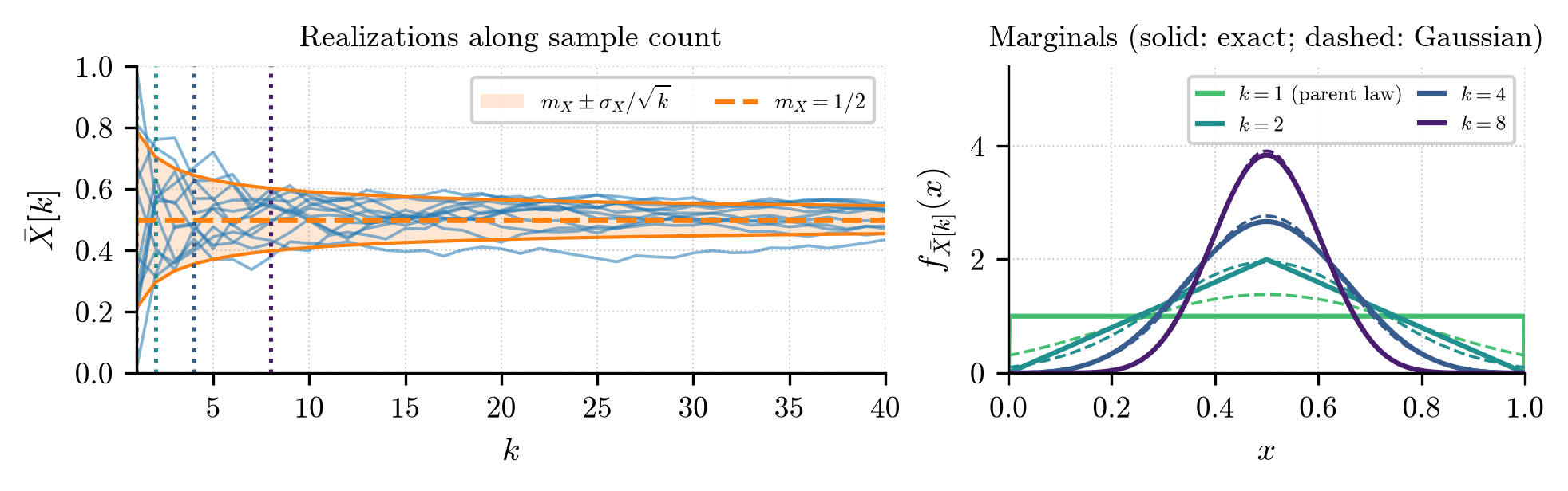
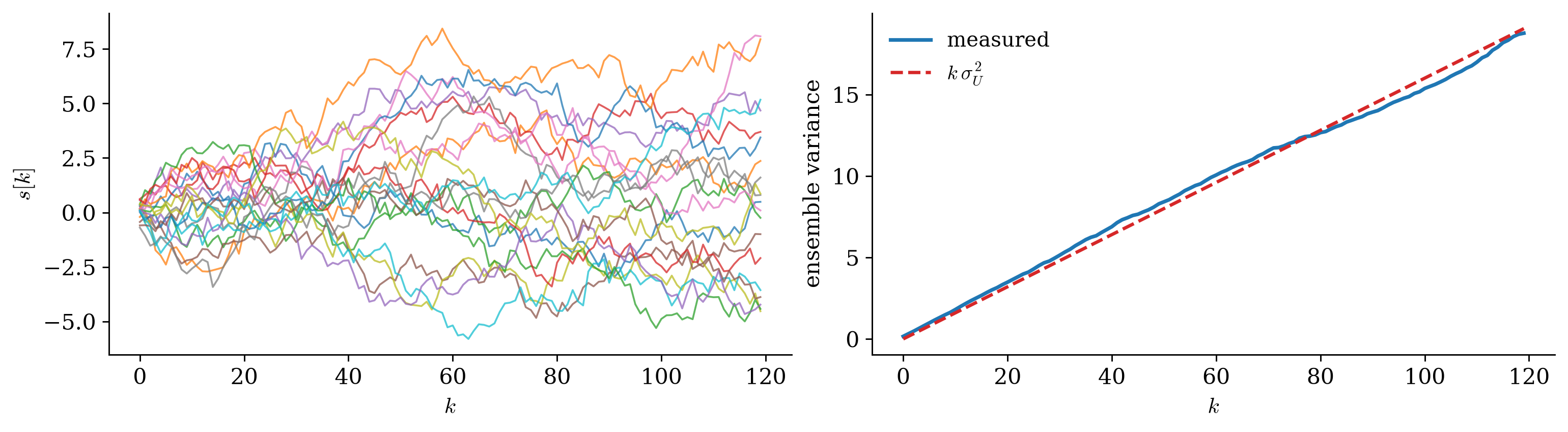
Read along time, each realization settles; read down the ensemble, the envelope closes as \(1/\sqrt k\). Every algorithm this week is a rule for how fast that envelope may be allowed to close.

The running mean

One quantity \(S\), measured \(k\) times with independent errors of variance \(\sigma_V^2\). The sample mean need not store the readings:

Running mean \[\widehat S[k]=\widehat S[k-1]+\frac1k\paren{X[k]-\widehat S[k-1]} .\]

The gain \(1/k\) is not a choice. With \(P[k-1]=\sigma_V^2/(k-1)\), \[\frac{P[k-1]}{P[k-1]+\sigma_V^2}=\frac1k:\] the ratio of what the estimate is unsure about to the total uncertainty of the new reading.

Old estimate + gain × innovation. The innovation \(X[k]-\widehat S[k-1]\) is the part of the new reading the old estimate could not predict.

Fusion, one measurement at a time

Fusion added precisions: \(\mathbf P^{-1}=\mathbf P_0^{-1}+\sum_i\mathbf H_i\herm\mathbf R_i^{-1}\mathbf H_i\). Split off the last sensor, treat everything before it as the prior, and the batch answer becomes a recursion:

Sequential fusion \[\widehat{\mathbf S}_i=\widehat{\mathbf S}_{i-1}+\mathbf K_i\,(\mathbf X_i-\mathbf H_i\widehat{\mathbf S}_{i-1}),\qquad \mathbf P_i=(\mathbf I-\mathbf K_i\mathbf H_i)\,\mathbf P_{i-1},\] \[\mathbf K_i=\mathbf P_{i-1}\mathbf H_i\herm\paren{\mathbf H_i\mathbf P_{i-1}\mathbf H_i\herm+\mathbf R_i}^{-1}=\mathbf P_i\mathbf H_i\herm\mathbf R_i^{-1}.\]

Only the last estimate and its covariance are carried. The answer after the last measurement is identical to the batch answer.

Repeated fixes, and fixes of unequal quality

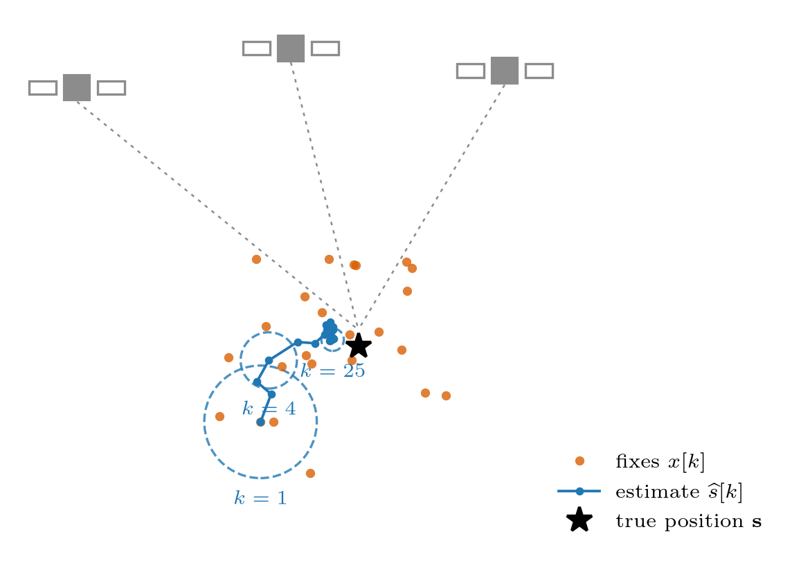
A fixed position \(\mathbf X[k]=\mathbf S+\mathbf V[k]\) with \(\mathbf R_{\mathbf{VV}}=\sigma_V^2\mathbf I\) and \(\mathbf H=\mathbf I\): the recursion is the running mean in each coordinate, and the uncertainty circle of the opening slide shrinks like \(1/\sqrt k\).

A fix taken with few satellites in view, or against a reflecting wall, is worth less. Give it its own \(\sigma_k^2\): the recursion is unchanged, and the result is the precision-weighted average of the Bayesian week. A worthless fix moves the estimate not at all, since its gain \(P/(P+\sigma_k^2)\to0\) by itself.

When the state moves

The running mean stops listening

Tracking a drifting position. Left: the fixes, the running mean, and predict-then-fuse. Right: their gains.

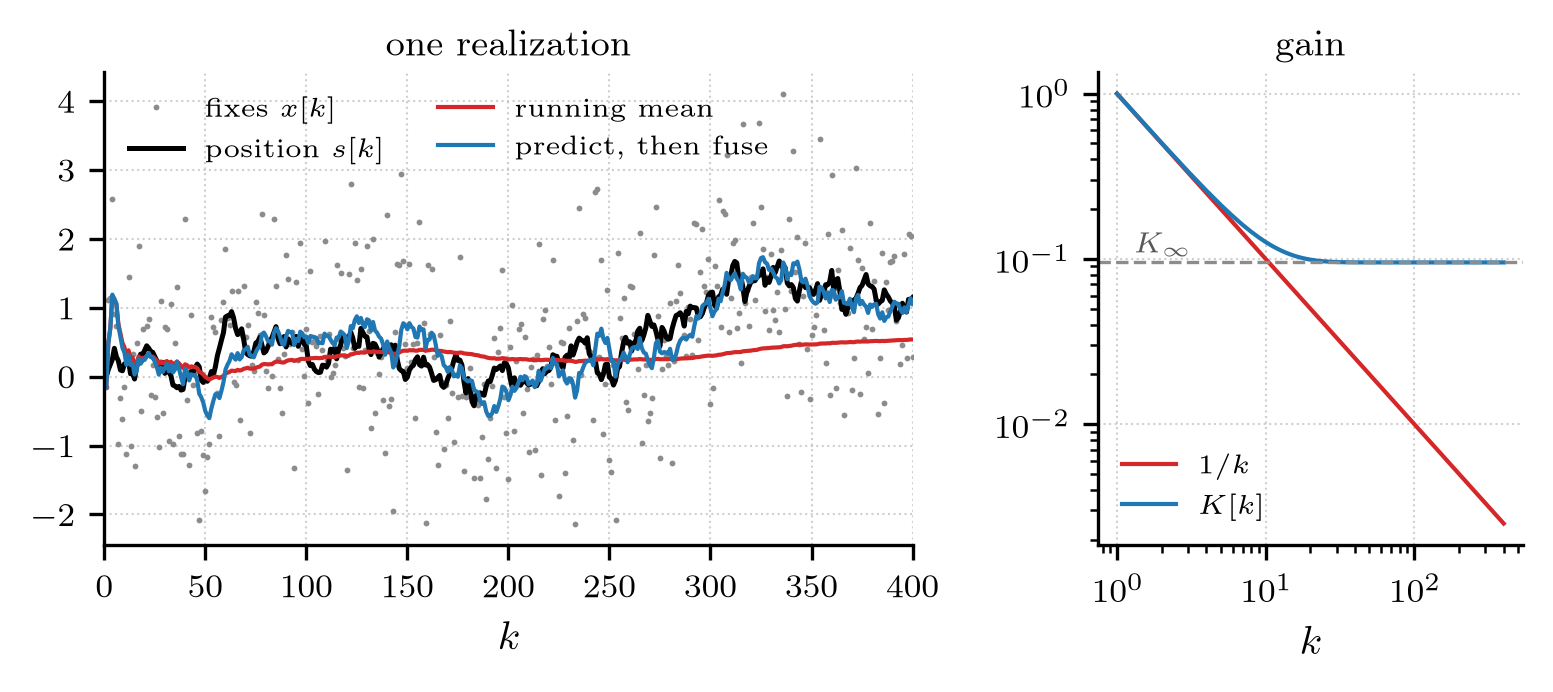
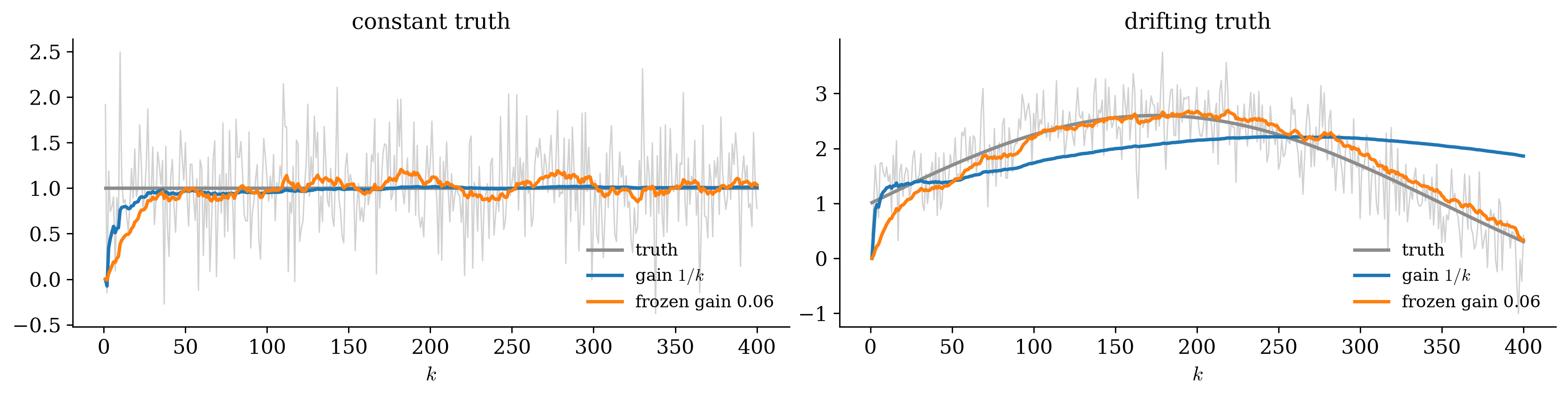
The running mean’s gain decays as \(1/k\): after a thousand fixes it barely moves, which is right for a fixed position and useless for a moving one.

Decaying gain against frozen gain

Figure 1: The same recursion on a constant and on a drifting truth, with the decaying gain 1/k and with a frozen gain μ = 0.06.

A decaying gain is optimal for a constant and useless for a drift. Two ways to keep up: let a model re-inflate the uncertainty (Kalman), or freeze the gain (every adaptive algorithm).

Predict, then fuse

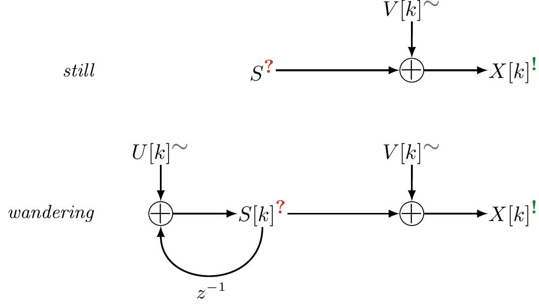
Let the position drift, \(S[k]=S[k-1]+U[k]\) with independent steps of variance \(\sigma_U^2\). Between two fixes the estimate cannot know where the step went:

Scalar Kalman filter

• Predict: \(\widehat S[k\mid k-1]=\widehat S[k-1\mid k-1]\), \(P[k\mid k-1]=P[k-1\mid k-1]+\sigma_U^2\).

• Fuse: the fix of variance \(\sigma_V^2\) with the prediction, with gain \(K=P[k\mid k-1]/\paren{P[k\mid k-1]+\sigma_V^2}\).

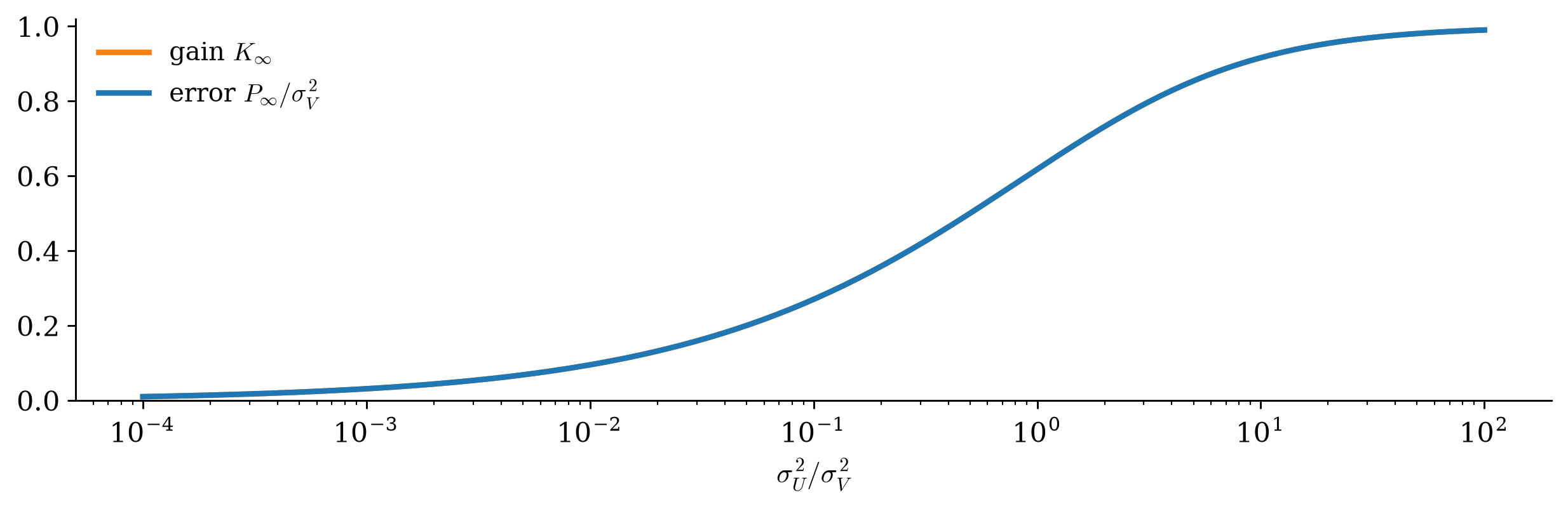
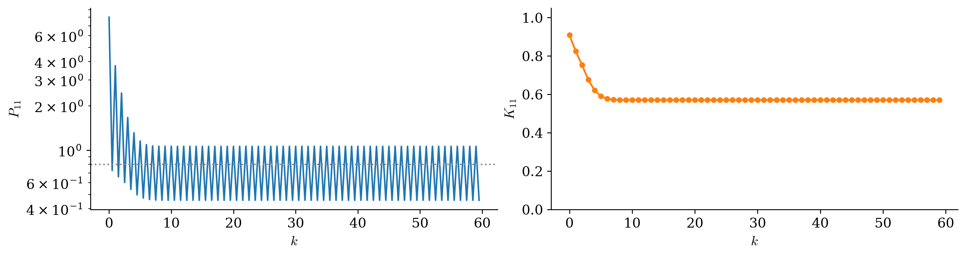
Uncertainty now grows between measurements, so the gain no longer dies. It settles at a constant \(K_\infty\), where what one fix removes equals what one step adds.

The steady-state gain

Figure 2: Steady-state gain K∞ and error variance P∞ of the scalar random-walk tracker, against the ratio of process to measurement noise q = σ_U²/σ_V².

A slow drift in a noisy sensor: small gain, long memory, heavy averaging. A fast drift or a clean sensor: gain near one, trust the latest fix. The ratio of two variances sets the memory of the tracker.

A random walk forgets nothing

Figure 3: Twenty realizations of a random walk, and the ensemble variance over 4000 realizations against kσ_U².

The model of a “constant that isn’t quite constant”: a wandering bias, a slowly moving target. Its variance grows without bound, which is why the estimator’s uncertainty must be allowed to grow too.

A random walk forgets nothing

Above, the state held still: the running mean. Below, the random walk: the only change is the return path.

The state-space model

\[\mathbf S[k]=\mathbf A\,\mathbf S[k-1]+\mathbf B\,\mathbf U[k],\qquad \mathbf X[k]=\mathbf H\,\mathbf S[k]+\mathbf V[k]\]

Both maps known, both noises random, the state sought. The loop through \(\mathbf A\) is what makes it a state.

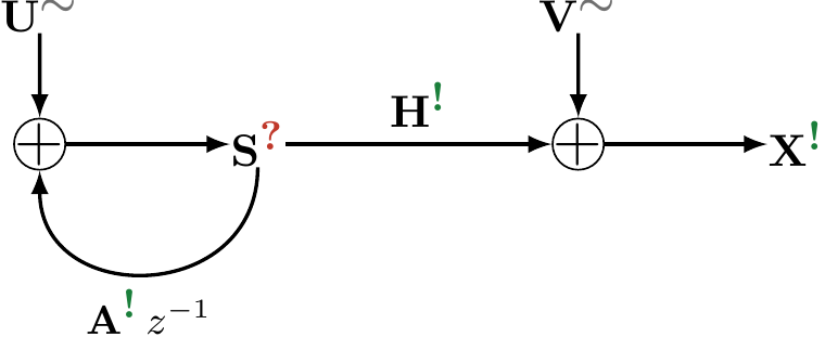
Two equations for two questions: how the unknown moves, and how it is seen. Keeping them apart is most of the conceptual work.

Two models of a moving train

Random walk: \(\mathbf A=1\); the model believes the train stays where it was.

Constant velocity State (position, velocity), random accelerations \(U\), sampling interval \(T\): \[S_p[k]=S_p[k-1]+T\,S_v[k-1]+\tfrac{T^2}{2}U[k],\qquad S_v[k]=S_v[k-1]+T\,U[k],\] \[\mathbf A=\begin{pmatrix}1&T\\0&1\end{pmatrix},\quad \mathbf B=\begin{pmatrix}T^2/2\\T\end{pmatrix},\quad \mathbf H=\begin{pmatrix}1&0\end{pmatrix}.\]

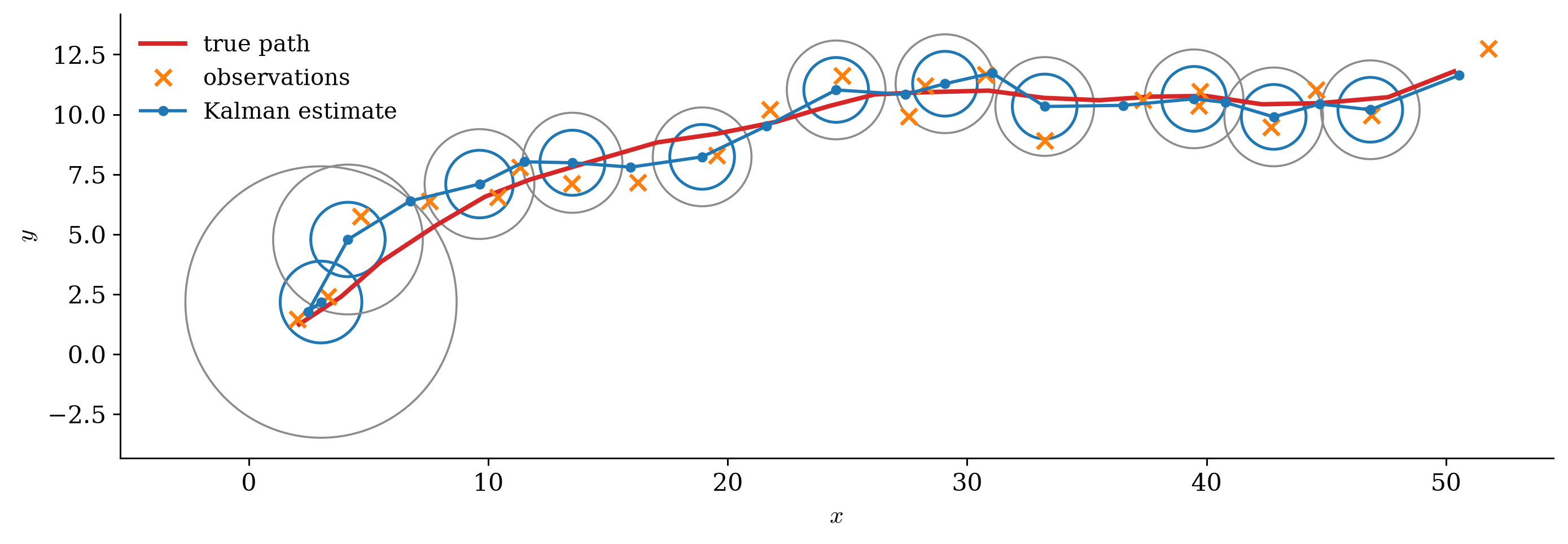
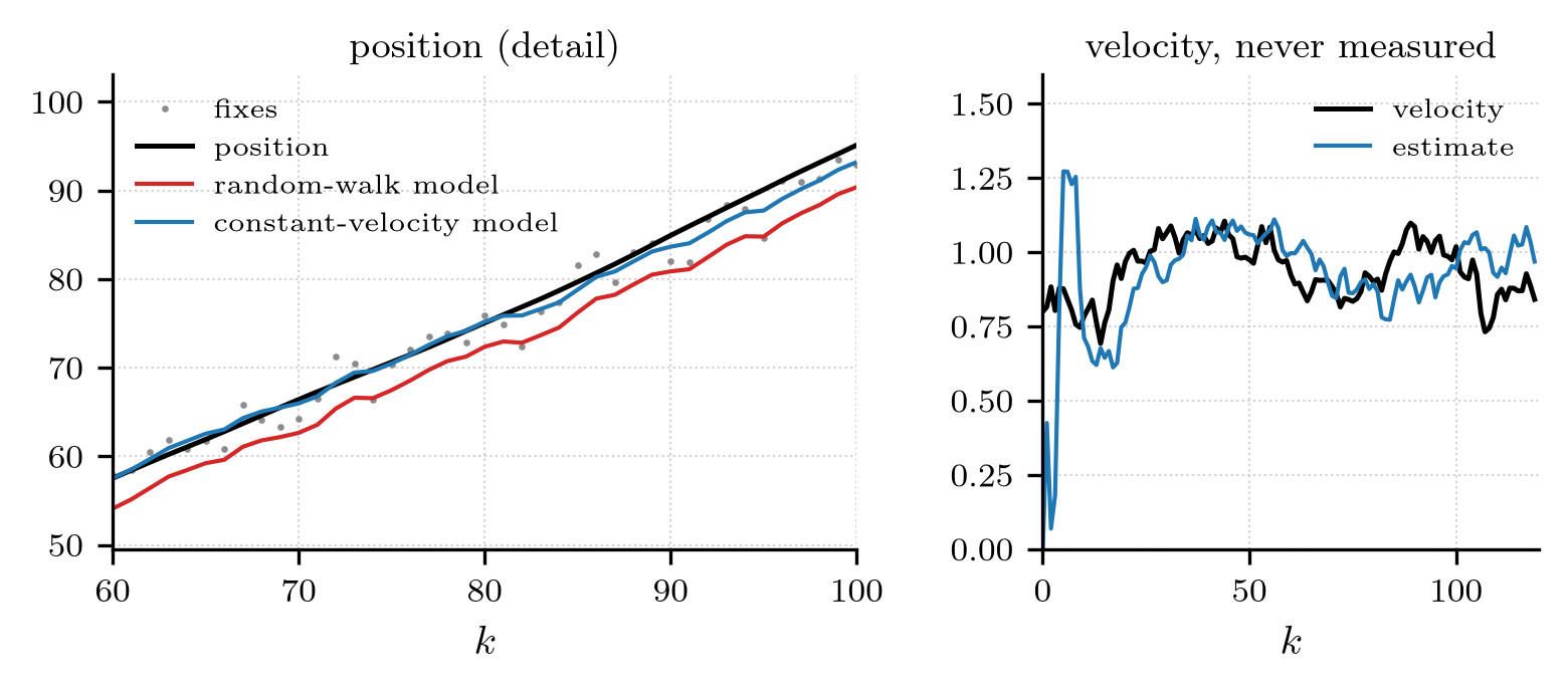
Only the position is measured. The velocity is a state nobody observes directly, and the filter will estimate it anyway.

The Kalman filter

Predict, then fuse, in matrices

Kalman filter Predict through the dynamics: \[\widehat{\mathbf S}[k|k-1]=\mathbf A\widehat{\mathbf S}[k-1|k-1],\qquad \mathbf P[k|k-1]=\mathbf A\mathbf P[k-1|k-1]\mathbf A\herm+\mathbf B\mathbf R_{\mathbf{UU}}\mathbf B\herm .\] Fuse the measurement, exactly as sequential fusion: \[\widehat{\mathbf S}[k|k]=\widehat{\mathbf S}[k|k-1]+\mathbf K[k]\,\bsy\nu[k],\qquad \mathbf P[k|k]=(\mathbf I-\mathbf K[k]\mathbf H)\,\mathbf P[k|k-1],\] \[\bsy\nu[k]=\mathbf X[k]-\mathbf H\widehat{\mathbf S}[k|k-1],\qquad \mathbf K[k]=\mathbf P[k|k-1]\mathbf H\herm\paren{\mathbf H\mathbf P[k|k-1]\mathbf H\herm+\mathbf R_{\mathbf{VV}}}^{-1}.\]

Every line is already derived

Nothing new in the Kalman filter

• Predict the estimate: linearity of expectation. Predict the covariance: \(\mathbf A\mathbf C\mathbf A\herm\) plus the fresh process noise.

• Fuse: sensor fusion with the prediction as prior, the affine MMSE estimator once per step.

Uncertain prediction: trust the data. Noisy sensor: trust the model. The gain decides, from the two covariances alone.

Why the recursion is optimal

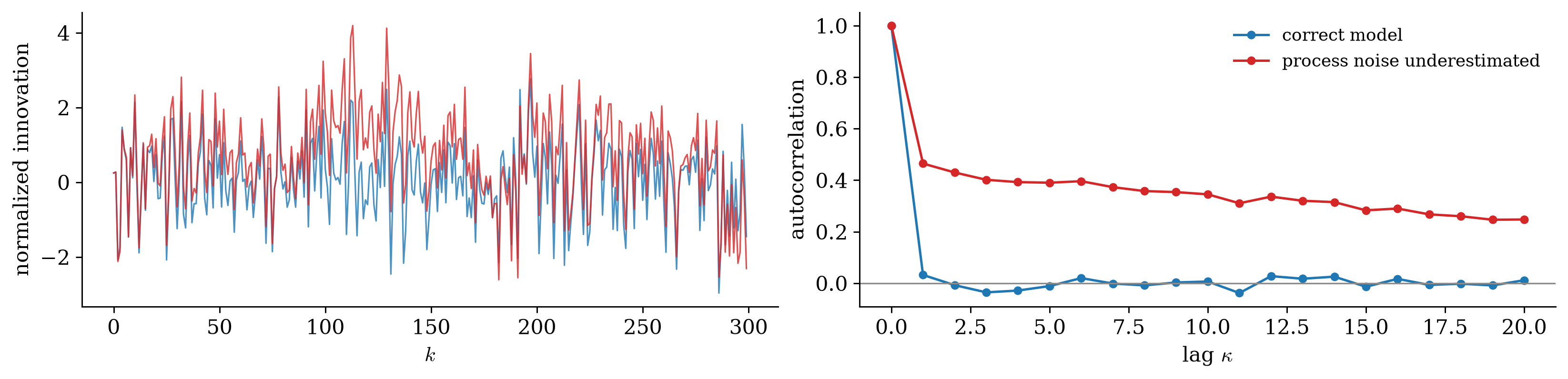
The innovations \(\bsy\nu[k]\) are white: each adds one new orthogonal direction, and updating along it is exact.

Optimality of the Kalman filter The best linear estimate of the state from all measurements so far, in constant memory. For Gaussian noise, the conditional mean \(\E{\mathbf S[k]\mid\mathbf X[1],\dots,\mathbf X[k]}\): the best estimate of any kind.

Nothing is approximated: the recursion reproduces the batch answer, it only refuses to recompute it.

Tracking a target

Figure 4: A constant-velocity target with random accelerations, observed in position only: the 2σ error ellipses after prediction (grey) and after the update (blue).

The gain settles, and so does the error

Figure 5: Left: the position error variance, growing at each prediction and shrinking at each update. Right: the Kalman gain converging to a constant.

The gain starts near one (the prior is worthless, trust the data) and converges to a fixed blend of model and measurement. The covariance and the gain do not depend on the data: they can be computed in advance.

The model matters

The same position fixes of a train, filtered with a random-walk model and with a constant-velocity model. Left: the random walk lags. Right: the velocity, estimated from position fixes alone.

The random-walk model predicts “it stays where it was” and falls behind by one interval’s travel at every step. The constant-velocity model predicts the motion, and estimates a velocity no sensor measured.

→ Demo: a Kalman tracker, its model, and its innovations

Checking a filter by its innovations

Figure 6: Normalized innovations of a scalar random-walk tracker over 2000 steps, and their sample autocorrelation, for the correct model and for a model that assumes the state moves 100 times less than it does.

Right model: white innovations of unit variance. Wrong model: correlated and too large, the filter keeps being surprised in the same direction. The innovations are the free diagnostic.

What the Kalman filter contains

Special cases

• The forecast of an AR process: the time update with no measurements.

• The Wiener filter: the steady state, when \(\mathbf P\) and \(\mathbf K\) converge.

• The running mean: \(\mathbf H=1\), no process noise, gain \(1/k\).

Told the most (a model of how the unknown moves), the Kalman filter is the most powerful and the most fragile: when the model is wrong, the advantage inverts.

When the unknown is a filter

The filter as a state

System identification read twice: as a static estimation problem, and as a state-space model whose state is the filter itself.

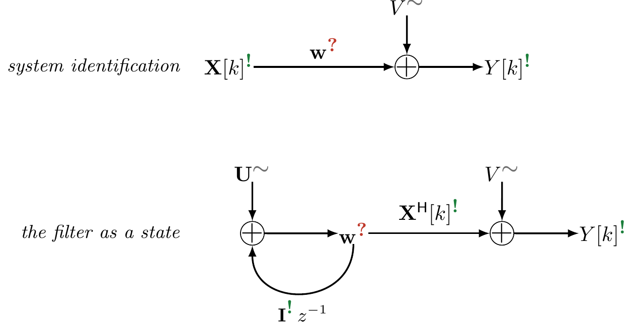
Let the state be the filter’s coefficients \(\mathbf w\), nearly constant (\(\mathbf A=\mathbf I\)), and let the measurement row be the input vector: \(Y[k]=\mathbf w\herm\mathbf X[k]+V[k]\). The Kalman filter on this model is recursive least squares (RLS).

Recursive least squares

RLS \[\mathbf g[k]=\frac{\beta^{-1}\mathbf P[k-1]\mathbf X[k]}{1+\beta^{-1}\mathbf X\herm[k]\mathbf P[k-1]\mathbf X[k]},\qquad \mathbf w[k]=\mathbf w[k-1]+\mathbf g[k]\,\xi\conj[k],\] \[\xi[k]=Y[k]-\mathbf w\herm[k-1]\mathbf X[k],\qquad \mathbf P[k]=\beta^{-1}\paren{\mathbf P[k-1]-\mathbf g[k]\mathbf X\herm[k]\mathbf P[k-1]}.\]

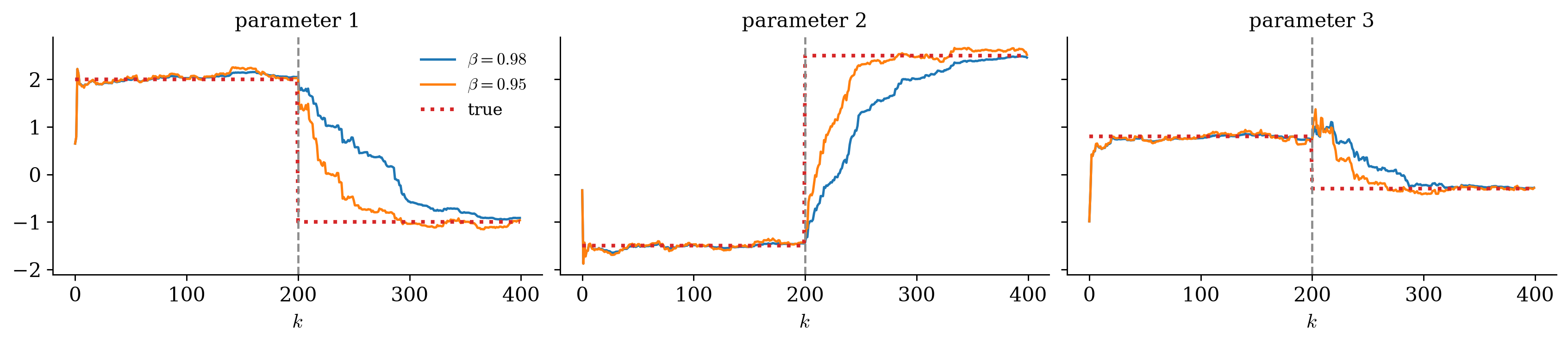
\(\mathbf P\) is the inverse of the exponentially weighted sample correlation of the inputs; the forgetting factor \(\beta<1\) re-inflates it, the role process noise plays in the Kalman filter.

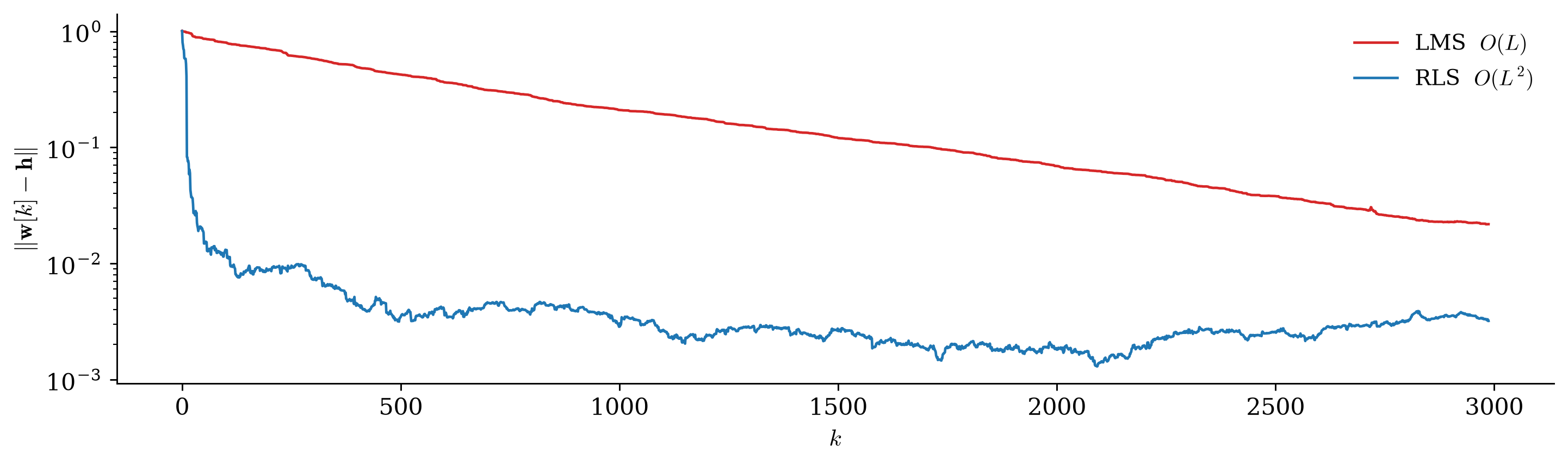
RLS converges in about a filter-length of samples, whatever the input. Its price is \(O(L^2)\) per sample: at \(L=256\) taps, about 65 000 multiplications per sample.

Forgetting: tracking against noise

Figure 7: Three parameters that jump at k = 200, tracked by RLS with two forgetting factors.

Stronger forgetting reacts faster to the change and is noisier once settled: the same bias–variance trade as every window length in the course.

Echo cancellation as a state-space problem

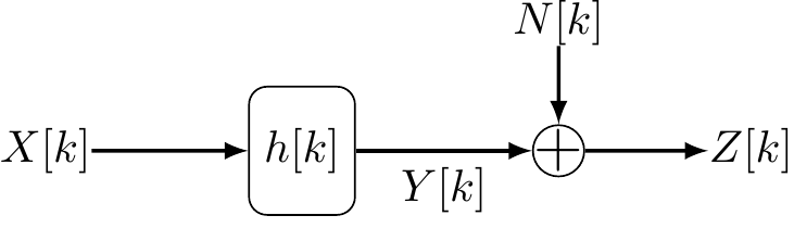
Hands-free telephony A loudspeaker plays the far-end signal \(X[k]\); the microphone picks up its echo through the room response \(\mathbf w\), plus the near-end talker, plus noise. The adaptive filter learns \(\mathbf w\) and subtracts the predicted echo.

Read as a state-space model: the room response is the state, drifting slowly as people move; the near-end talker is measurement noise.

When the near end talks, the measurement noise is large and the Kalman gain shrinks by itself: the filter stops adapting. Double-talk detection is a noise-variance estimator.

The echo canceller

The error the algorithm minimizes is exactly the signal the far end hears. When the near end talks, that error is large for a reason the filter must not learn from.

The other route: follow the gradient

The error surface is a bowl

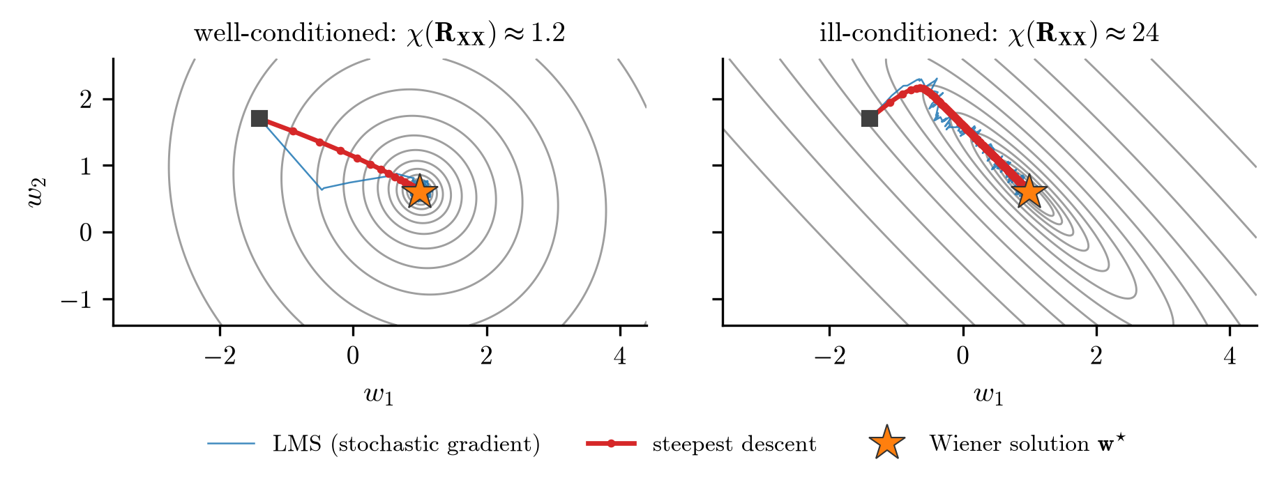
\(J(\mathbf w)=\E{\abs{Y-\mathbf w\herm\mathbf X}^2}\) is a quadratic bowl with its bottom at the Wiener solution, and contours shaped by \(\mathbf R_{\mathbf{XX}}\). Steepest descent slides down it: \[\mathbf w[k+1]=\mathbf w[k]+\mu\paren{\mathbf r_{\mathbf{XY}}-\mathbf R_{\mathbf{XX}}\mathbf w[k]} .\]

Convergence of steepest descent It converges to \(\mathbf w\opt\) from any start if and only if \(0<\mu<2/\lambda_{\max}\); the mode along eigenvalue \(\lambda_i\) decays as \((1-\mu\lambda_i)^k\).

It still needs \(\mathbf R_{\mathbf{XX}}\) and \(\mathbf r_{\mathbf{XY}}\): the statistics-known ideal the practical algorithms approximate.

The eigenvalue spread sets the pace

Contours of the error surface of a two-tap filter and the descent, for a near-white and a strongly colored input.

The step is capped by \(\lambda_{\max}\), so the slowest mode crawls at the rate \(\lambda_{\min}/\lambda_{\max}\). For a stationary input that spread is bounded by the dynamic range of the spectrum: a peaky spectrum makes a long, narrow valley.

A peaky spectrum, in numbers

AR(1) input For an input with pole \(\rho\) the spectrum runs between \(1/(1+\rho)^2\) and \(1/(1-\rho)^2\), so the eigenvalue spread approaches \(\paren{\frac{1+\rho}{1-\rho}}^2\). At \(\rho=0.9\) that is about \(361\).

Stability forces \(\mu<2/\lambda_{\max}\), and the slowest mode then needs at least \(\lambda_{\max}/(2\lambda_{\min})\approx180\) times as many iterations as the fastest, whatever \(\mu\) is chosen.

The input decides the convergence speed, not the tuning. The same number conditioned the normal equations of estimation-as-projection.

LMS: drop the expectation

LMS \[\mathbf w[k+1]=\mathbf w[k]+\mu\,\mathbf X[k]\,e\conj[k],\qquad e[k]=Y[k]-\mathbf w\herm[k]\mathbf X[k].\]

Replace the unknown gradient by its one-sample estimate. Taking expectations, \(\E{\mathbf Xe\conj}=\mathbf r_{\mathbf{XY}}-\mathbf R_{\mathbf{XX}}\mathbf w\): LMS in the mean is steepest descent, with the same \(\mu\) and the same stability bound (under the independence assumption between weights and data).

It needs no statistics at all, two multiply-adds per tap, and is the most widely deployed adaptive filter there is. The price is gradient noise: it fluctuates around the Wiener solution, the misadjustment.

LMS against RLS

Figure 8: Identifying the same 12-tap system from a strongly colored input (AR(1), pole at 0.92).

RLS whitens as it goes and does not care about the spread; LMS crawls down the valley. Samples against operations: two different currencies.

NLMS: independent of the input level

Divide the step by the input energy, \(\mathbf w[k+1]=\mathbf w[k]+\frac{\tilde\mu}{\varepsilon+\norm{\mathbf X[k]}^2}\mathbf X[k]e\conj[k]\), \(0<\tilde\mu<2\):

Figure 9: The same identification with the input level raised tenfold halfway through. LMS, tuned on the quiet part, goes unstable; NLMS is unaffected.

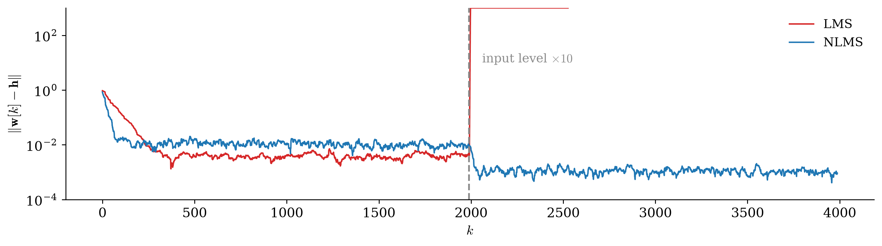
The normalized step is dimensionless, so its stability range no longer depends on the signal level. The regularizer \(\varepsilon\) is not a formality: in a speech pause \(\mathbf X\approx\mathbf0\) and the quotient would blow up.

Gradient methods are frozen Kalman filters

Freeze the Kalman covariance at \(p\,\mathbf I\) and never update it. The RLS gain becomes \[\mathbf g[k]=\frac{\mathbf X[k]}{\norm{\mathbf X[k]}^2+\sigma_V^2/p} \;\longrightarrow\;\frac{p}{\sigma_V^2}\,\mathbf X[k]:\] NLMS with \(\varepsilon=\sigma_V^2/p\), and in the limit LMS with \(\mu=p/\sigma_V^2\).

what is thrown away	what it costs
\(\mathbf P\) isotropic, not shaped by the input	convergence limited by \(\lambda_{\max}/\lambda_{\min}\)
\(\mathbf P\) never reduced by measurements	the gain never decays: misadjustment
\(\sigma_V^2\) constant, not estimated	no automatic slowdown when the near end talks

What each algorithm is told

algorithm	is told	cost per step	convergence
steepest descent	\(\mathbf R_{\mathbf{XX}}\), \(\mathbf r_{\mathbf{XY}}\)	—	spread-limited; the ideal
LMS	nothing	\(O(L)\)	slow, spread-limited
NLMS	nothing	\(O(L)\)	slow, level-robust
RLS	nothing, estimates \(\mathbf R_{\mathbf{XX}}\) as it goes	\(O(L^2)\)	fast, spread-free
Kalman	a model of how the state moves	\(O(M^3)\)	optimal if the model holds

A story about information, not cleverness: every row descends the same bowl, and pays for what it is not told.

The isotropic assumption of LMS is also a refusal to over-claim: an estimator that never claimed to know its uncertainty cannot be confidently wrong about it.

One projection

A space with an inner product

A Hilbert space is a (complete) vector space with an inner product. That is all.

space	elements	\(\ip{x,y}\)	orthogonal means
randomness	random variables	\(\E{XY\conj}\)	uncorrelated
time	finite-energy sequences	\(\sum_kx[k]y\conj[k]\)	no overlap in time
sensors	array snapshots	\(\mathbf y\herm\mathbf x\)	spatially orthogonal
frequency	spectra	\(\frac{1}{2\pi}\int XY\conj\dd\Omega\)	disjoint bands

Choosing a Hilbert space is choosing what “similar” means for the problem. The estimator, its error and its algorithm all follow from that one choice.

An orthonormal basis hands back the coordinates

Orthonormal expansion For \(\ip{e_i,e_j}=\delta_{ij}\): \(a_i=\ip{x,e_i}\), and \(\norm{x}^2=\sum_i\abs{a_i}^2\) (Parseval). No system to solve.

In \(\Complex^n\) the coordinate vector; for sequences, the DFT; for spectra, the Fourier series; for random variables in the eigenbasis of their covariance, the KLT.

So much of the course was spent manufacturing orthogonality: by rotation, by whitening, by prediction, by the Fourier transform.

Nine weeks, one equation

For generators that are not orthonormal, the projection solves \(\mathbf G\,\mathbf a=\mathbf b\) with \(G_{ij}=\ip{x_i,x_j}\) and \(b_i=\ip{y,x_i}\). Only the inner product changes.

Figure 10: Gram matrices of four estimators, each from its own inner product. All four go to the same line of code, a = solve(G, b).

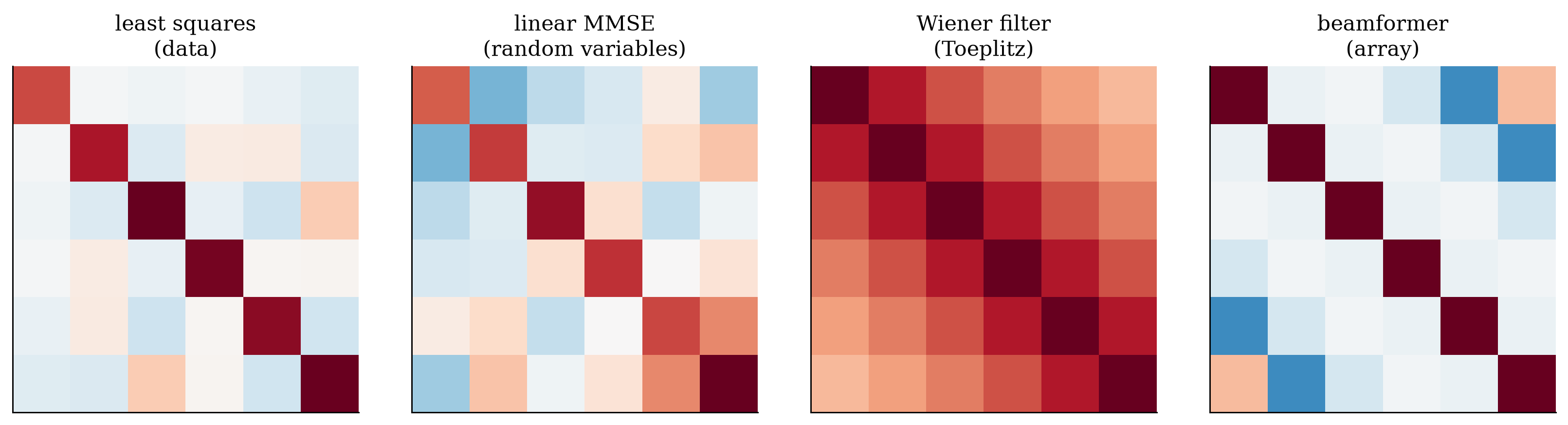
\(\mathbf G^{-1}\) always does the same job: it undoes what the observations share, whether that is called collinearity, correlation, coloring in time, or the signature of an interferer.

The one estimate that escapes

Every estimator above projected onto a linear span. One did not: the conditional mean \(\E{Y\mid\mathbf X}\) is the projection onto all functions of the data.

It is the best estimate there is, but needs the whole joint law. The linear projections need only second moments, and give up the gap between the two.

Under a Gaussian model the gap is zero That single fact is why this course could be built on second moments and still be optimal.

Where the course lives

level	the object	the estimate	the equation
one number	a random variable	a parameter from a sample	likelihood, posterior
finitely many	a random vector	one variable from others	\(\mathbf R_{\mathbf{XX}}\mathbf w=\mathbf r_{\mathbf{XY}}\)
a signal	a stationary process	a signal from a signal	Wiener–Hopf, \(h*R_{XX}=R_{YX}\)
a moving signal	a state	the state, recursively	predict, then fuse

One idea met at four sizes: the best estimate is the orthogonal projection onto what you have observed. Everything else is choosing the space, and computing the projection efficiently.

Recap

This week

1. Recursive fusion carries only an estimate and its covariance. A moving state needs its uncertainty to grow between measurements: predict, then fuse. That is the Kalman filter; it is exact, and the model decides how good it is.

2. When the unknown is a filter, the Kalman filter is RLS: fast, \(O(L^2)\). Steepest descent, LMS and NLMS follow the gradient of the same bowl, cheap and slowed by the eigenvalue spread; they are the Kalman recursion with its covariance frozen.

3. Every estimator in the course is one projection, \(\mathbf G\mathbf a=\mathbf b\); only the inner product changes.