Estimators, detectors, and the floor no estimator beats
\[ % Number sets \newcommand{\Nat}{\mathbb{N}} \newcommand{\Integer}{\mathbb{Z}} \newcommand{\Real}{\mathbb{R}} \newcommand{\Complex}{\mathbb{C}} % Operators \newcommand{\SNR}{\operatorname{SNR}} \newcommand{\tr}{\operatorname{tr}} \newcommand{\re}{\operatorname{Re}} \newcommand{\im}{\operatorname{Im}} \newcommand{\sign}{\operatorname{sign}} \newcommand{\rect}{\operatorname{rect}} \newcommand{\sinc}{\operatorname{si}} \newcommand{\erf}{\operatorname{erf}} \newcommand{\erfc}{\operatorname{erfc}} \newcommand{\kurt}{\operatorname{kurt}} \newcommand{\diag}{\operatorname{diag}} \newcommand{\MSE}{\operatorname{MSE}} \newcommand{\argmin}{\operatorname*{argmin}} \newcommand{\argmax}{\operatorname*{argmax}} \newcommand{\bias}{\operatorname{bias}} \newcommand{\Bin}{\operatorname{Bin}} % Delimiters \newcommand{\paren}[1]{\left(#1\right)} \newcommand{\bracket}[1]{\left[#1\right]} \newcommand{\set}[1]{\left\{#1\right\}} \newcommand{\abs}[1]{\left\lvert #1 \right\rvert} \newcommand{\norm}[1]{\left\lVert #1 \right\rVert} \newcommand{\ip}[1]{\left\langle #1 \right\rangle} % Notation \newcommand{\dd}{\,\mathrm{d}} \newcommand{\tran}{^{\top}} \newcommand{\conv}{\ast} \newcommand{\conj}{^{*}} \newcommand{\herm}{^{\mathsf{H}}} \newcommand{\opt}{^{\star}} % Expectation and variance % \newcommand{\E}[1]{\mathbb{E}\!\left[#1\right]} \newcommand{\E}[2][]{\mathbb{E}_{#1}\!\left[#2\right]} \newcommand{\Var}[1]{\mathbb{V}\!\left[#1\right]} % Distributions \newcommand{\Gauss}{\mathcal{N}} \newcommand{\Uniform}{\mathcal{U}} \newcommand{\FT}{\mathcal{F}} % Probability \newcommand{\Prob}[1]{\mathbb{P}\!\left(#1\right)} % Misc \newcommand{\bsy}[1]{\boldsymbol{#1}} \newcommand{\calR}{\mathcal{R}} \newcommand{\calC}{\mathcal{C}} \]
How long did the run last? A production line stamps each item with the time it was made, in hours from the start of the run. The run lasted \(\phi\) hours, so the time stamps are spread over \([0,\phi]\). You have seen five, drawn at random: \[3.1,\quad 7.2,\quad 9.9,\quad 12.4,\quad 19.8 \qquad (\text{uniform on } [0,\phi]).\] How large is \(\phi\)?
More than one answer is defensible. Which is best, and is there a best possible? This week turns those two questions into mathematics.
Estimators. Any function of the data, itself a random variable, judged by its bias and variance.
Detectors. The unknown takes only two values; the optimal statistic is the likelihood ratio.
Maximum likelihood and the floor. The same comparison over all candidate values, and the Cramér–Rao bound that no unbiased estimator beats.
In the notes Estimation within Statistics · Point Estimation and Quality Criteria · Hypothesis Testing and Detection · Maximum Likelihood Estimation · The Cramér–Rao Bound
Probability runs forward, from a model to the data it generates. Statistics runs backward, from data to the model.
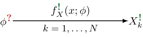
The data are an iid sample whose law belongs to a parametric family with unknown parameter \(\phi\): \[f(\mathbf x;\phi)=\prod_{k=1}^N f_X(x_k;\phi).\] The semicolon says \(\phi\) is unknown but fixed: not random, and with no distribution of its own.
Estimator Any function of the data, \(\widehat\Phi=\Theta(X_1,\dots,X_N)\). Built from random data, it is itself a random variable, and its distribution is how we judge it.
What is the frequency of this tone?
Answer two questions in the poll, without talking to your neighbors:


| predicted spread (class median of Q2) | ___ Hz |
| observed spread \(s\) | ___ Hz |
| class average \(\bar x\) | ___ Hz |
| its standard error \(s/\sqrt N\) | ___ Hz |
The tone was \(\theta=789\) Hz.
\[\underbrace{\tfrac1N\sum_i (x_i-\theta)^2}_{\text{error}} =\underbrace{\tfrac1N\sum_i (x_i-\bar x)^2}_{\text{spread}} +\underbrace{(\bar x-\theta)^2}_{\text{bias}^2}\]
The spread was measurable before the reveal. The bias was not.
Was \(\abs{\bar x-\theta}\) within a few \(s/\sqrt N\)? If not, we were all wrong in the same direction, and a bigger class would not have helped.
Estimator quality \[\text{bias}=\E{\widehat\Phi}-\phi,\qquad \MSE=\E{(\widehat\Phi-\phi)^2}=\Var{\widehat\Phi}+\text{bias}^2 .\]
All three are read at a fixed \(N\). As \(N\) grows: asymptotically unbiased if the bias vanishes, consistent if \(\widehat\Phi\to\phi\), which needs both terms of the MSE to vanish.
Unbiasedness is not the goal; small error is. A little bias that buys a lot of variance is a good trade, and a deliberate one.
Insert the estimator’s own mean and expand, exactly as for the best constant guess: \[\E{(\widehat\Phi-\phi)^2} =\E{(\widehat\Phi-\E{\widehat\Phi})^2} +2\,\underbrace{\E{\widehat\Phi-\E{\widehat\Phi}}}_{=0}\,(\E{\widehat\Phi}-\phi) +(\E{\widehat\Phi}-\phi)^2 .\]
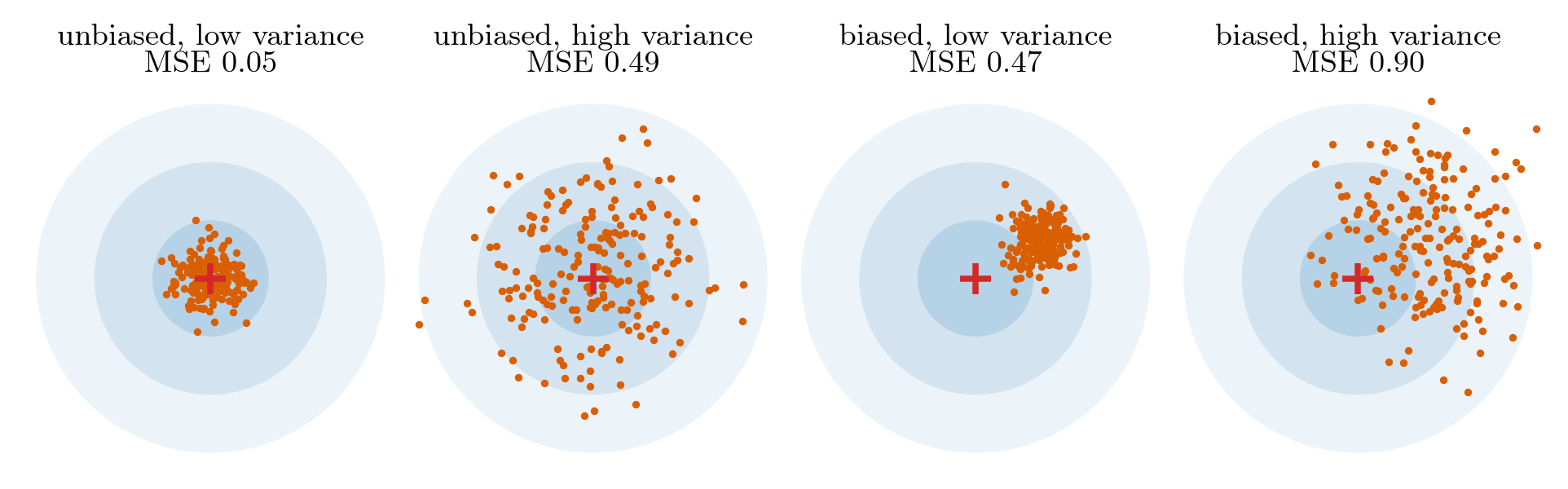
Variance: how much the estimate wobbles from sample to sample. Bias: where it wobbles around. A dartboard with a tight cluster off-center, and a wide cluster on-center.
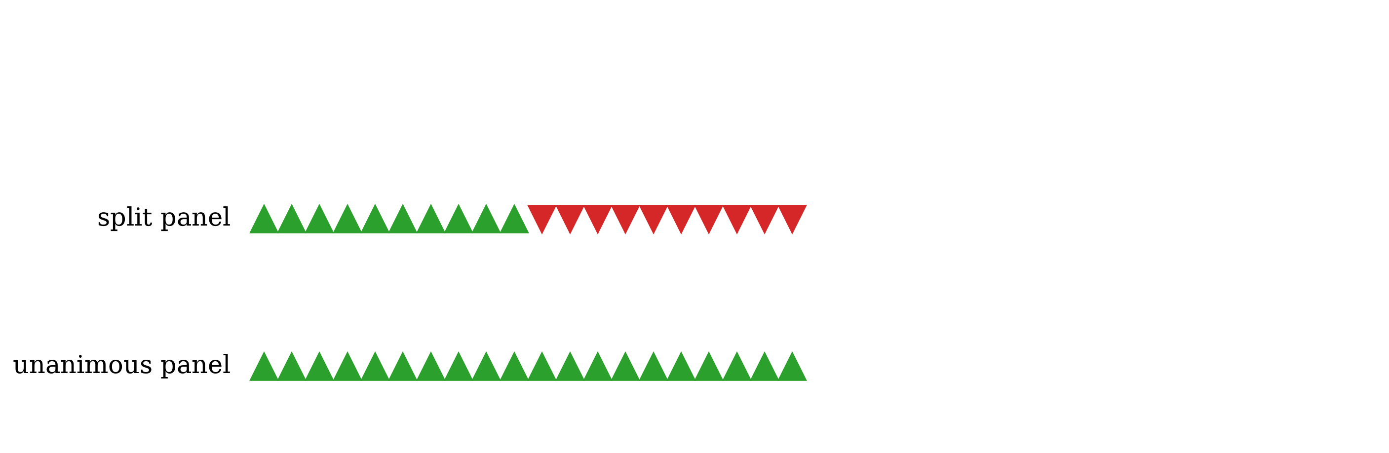
Two panels of twenty economists each forecast whether the economy grows next year (1) or shrinks (0).
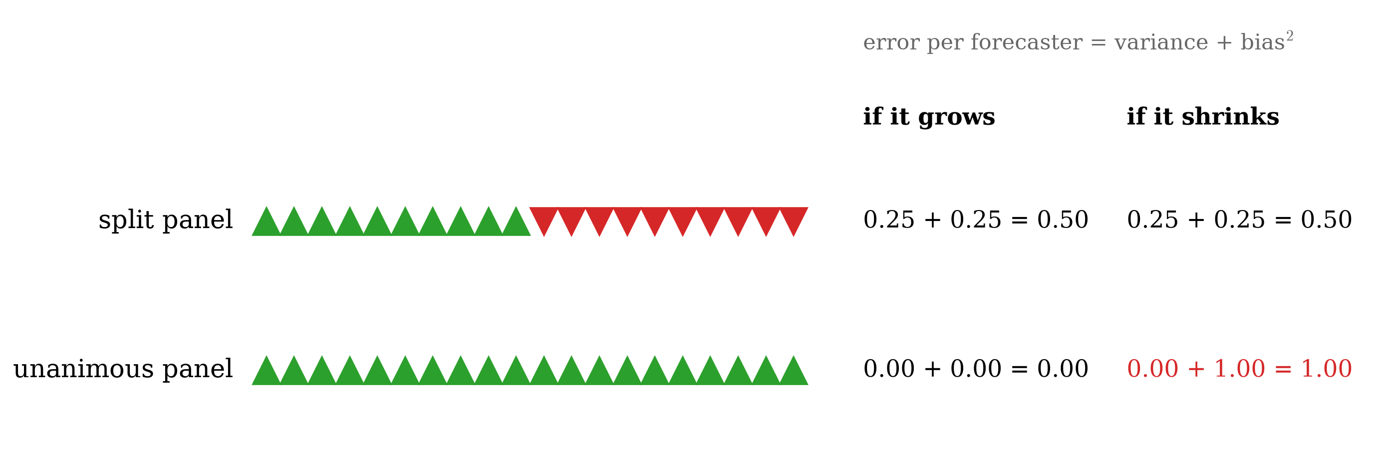

Split: half are wrong whatever happens, and we know it today. Unanimous: error \(0\) or \(1\), and only the outcome will tell.
Variance (noise) is measured from the estimates alone; bias needs the truth.

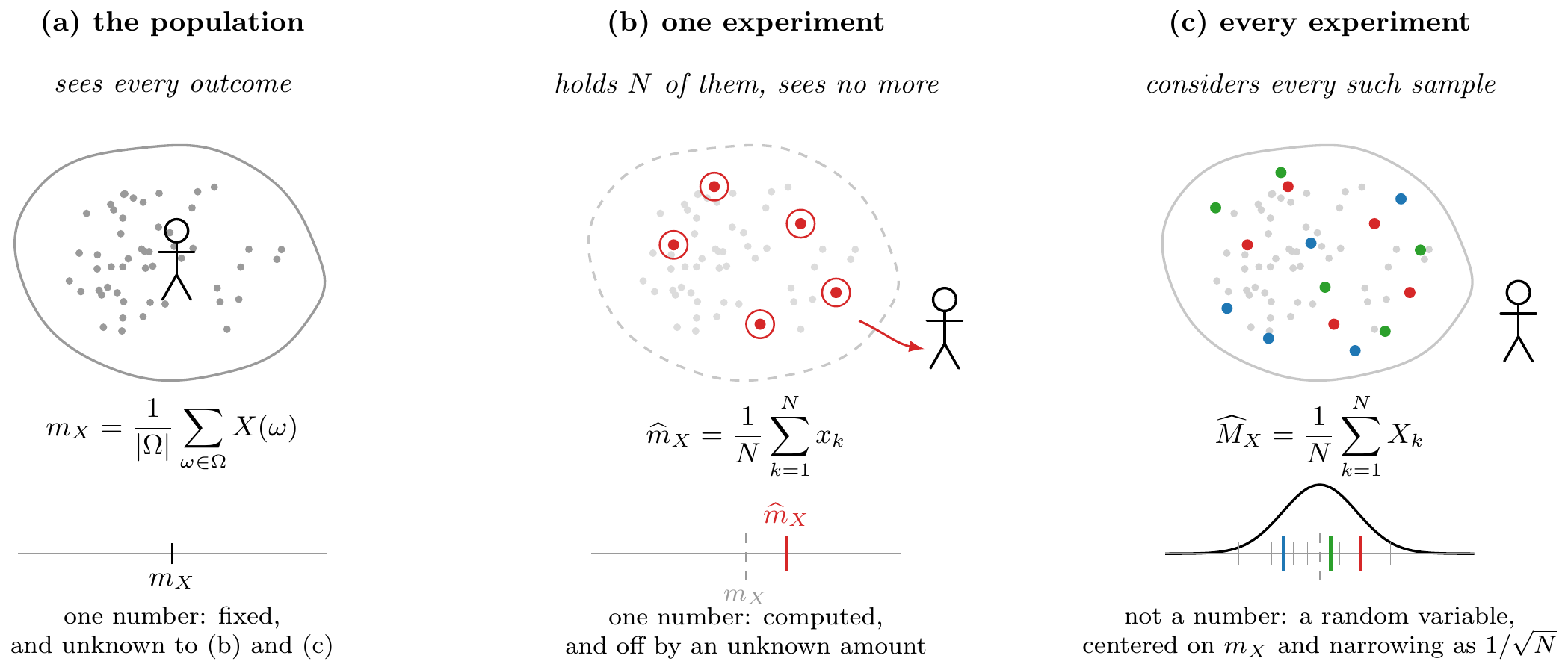
\(\widehat M_X=\frac1N\sum_kX_k\) is unbiased by linearity, at every \(N\), and has variance \(\sigma_X^2/N\). So it is consistent (the law of large numbers, read as a fact about an estimator), and by the central limit theorem its whole sampling distribution is known: \[\widehat M_X\approx\Gauss\!\paren{m_X,\tfrac{\sigma_X^2}{N}} .\]
None of this assumed a distribution for the data: only a finite variance. It is the yardstick every other estimator is measured against.
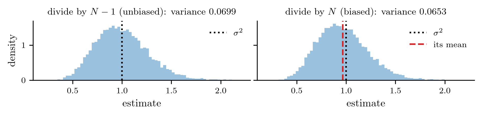
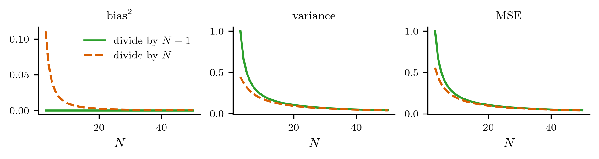
With the mean known, \(\frac1N\sum_k(X_k-m_X)^2\) is unbiased. With the mean estimated from the same data it is not: \[\E{\frac1N\sum_{k=1}^N(X_k-\widehat M_X)^2}=\frac{N-1}{N}\,\sigma_X^2, \qquad\text{so use}\qquad \widehat\Sigma_X^2=\frac{1}{N-1}\sum_{k=1}^N(X_k-\widehat M_X)^2 .\]
\(\widehat M_X\) is by construction the point closest to the data, so the residuals around it are too small. Fitting the mean uses up one of the \(N\) directions the data could vary in: \(N-1\) degrees of freedom remain.


Method of moments With \(p\) unknown parameters, set \(\frac1N\sum_k x_k^n=\E{X^n;\phi}\) for \(n=1,\dots,p\) and solve.
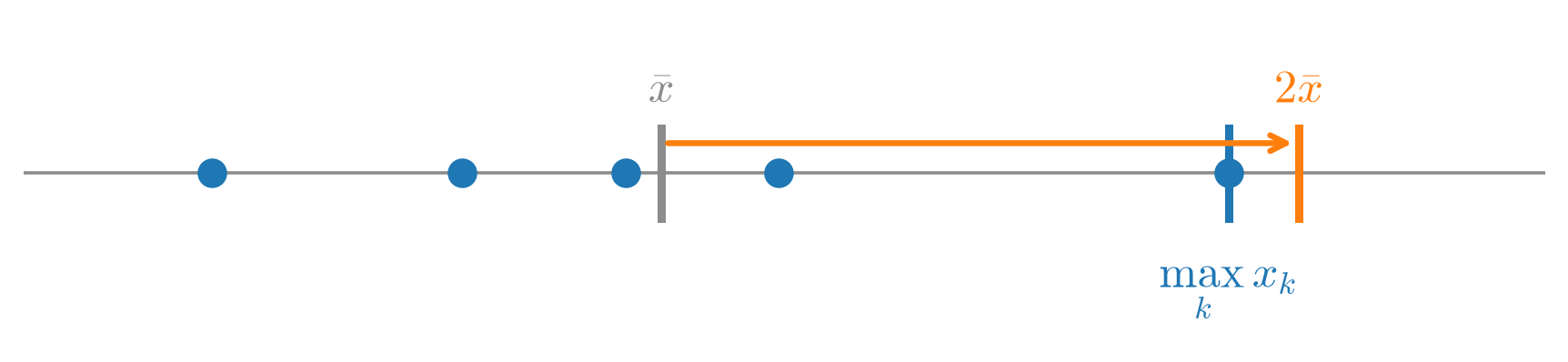
The puzzle (\(p=1\)). The model mean is \(\phi/2\), so \[\widehat\phi_{\text{MoM}}=\frac2N\sum_kx_k=20.96,\] the twice the average guess: unbiased, consistent, one moment.
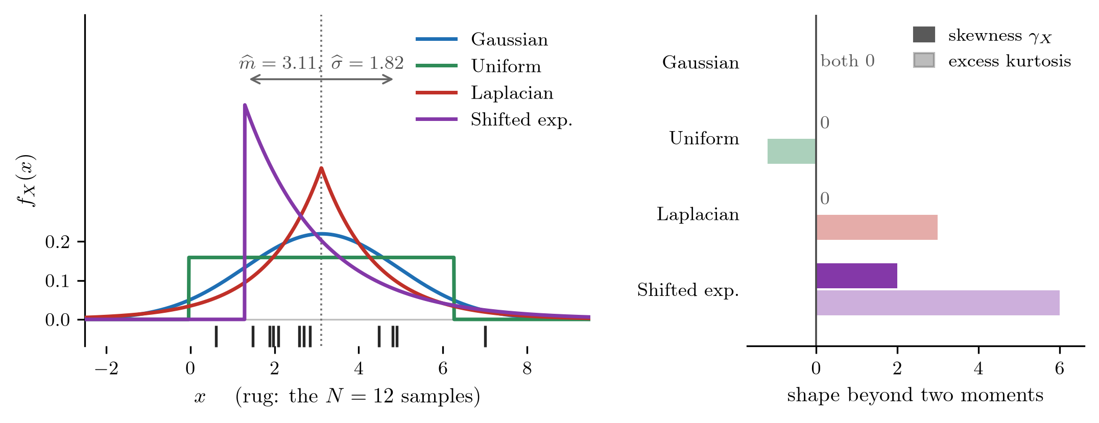
A Gaussian (\(p=2\)). Matching \(\E{X}\) and \(\E{X^2}\) gives \[\widehat m=\bar x,\qquad \widehat\sigma^2=\frac1N\sum_k(x_k-\bar x)^2,\] the divide-by-\(N\) estimator of the last slide.
Suspiciously wasteful: it reads only the average, while a sample near the edge says far more about where the edge is. The rest of the week explains how much it throws away.

The fits differ only in the higher moments, which twelve points estimate very badly. Matching moments answers the questions you asked of it, and no others.
The parameter takes only two values, \(H_0\) and \(H_1\), and the answer must be one of them, with no option to hedge.

With two answers there is no estimator distribution to track: the whole problem is which data lead to which answer.
A decision rule is fixed by its decision regions: decide \(H_1\) if \(\mathbf x\in\mathcal X_1\), \(H_0\) if \(\mathbf x\in\mathcal X_0\).
| decide \(H_0\) | decide \(H_1\) | |
|---|---|---|
| \(H_0\) true | correct silence | false alarm \(P_F\) |
| \(H_1\) true | miss \(1-P_D\) | detection \(P_D\) |
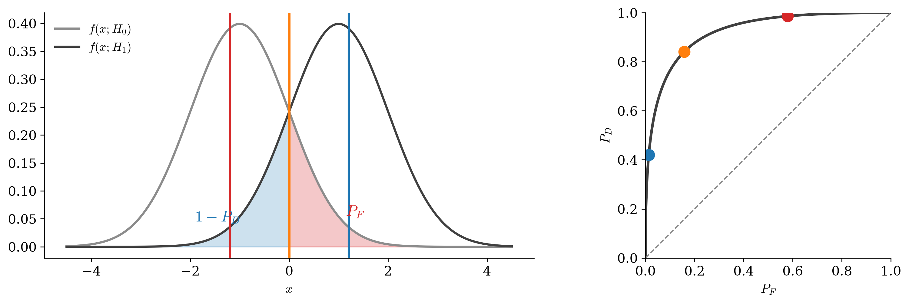
Each row sums to one, so two numbers describe any rule completely, and they pull against each other: fewer false alarms buys more misses.
Type I and Type II in statistics, false alarm and miss in radar, false positive and false negative in medicine: the same table.
Threshold a test statistic: \(\Theta(\mathbf x)\gtrless t\), so that \(\mathcal X_1=\set{\mathbf x:\Theta(\mathbf x)>t}\).
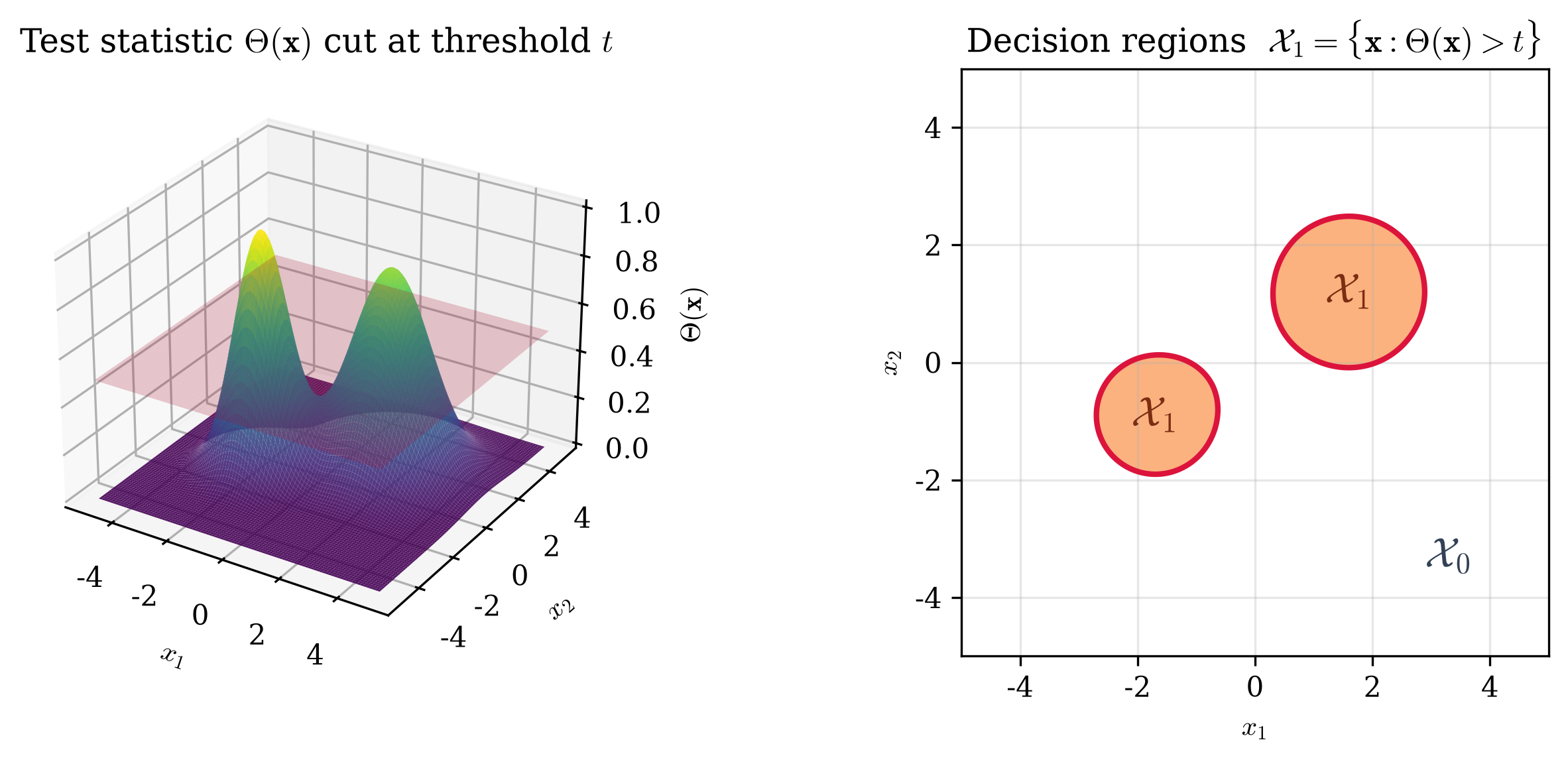
A statistic collapses \(N\)-dimensional data onto one axis, so the region becomes an interval. The question is which statistic.
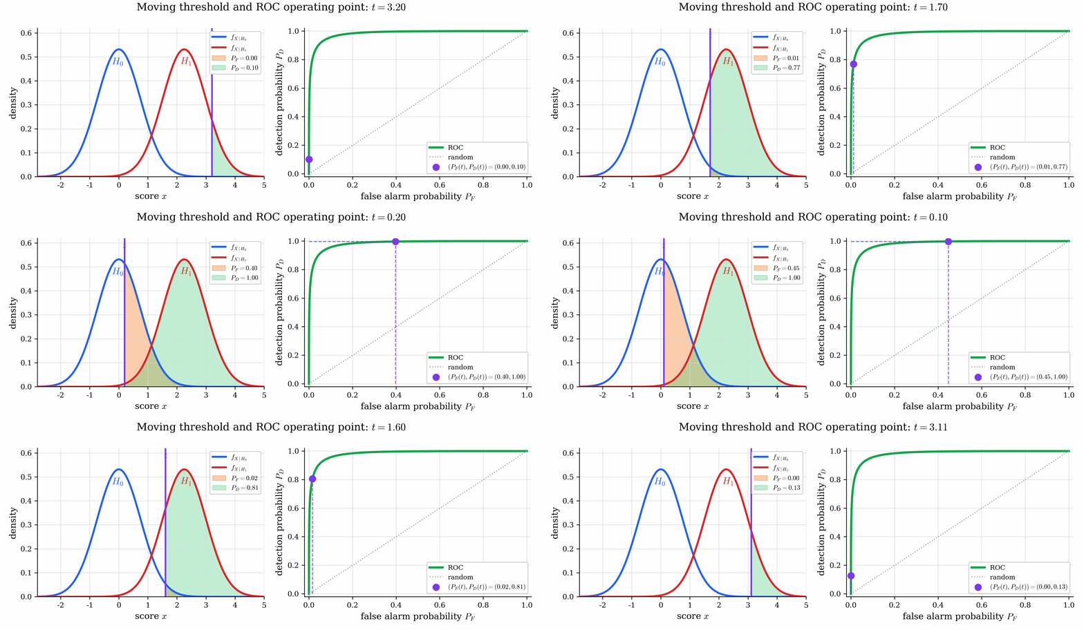
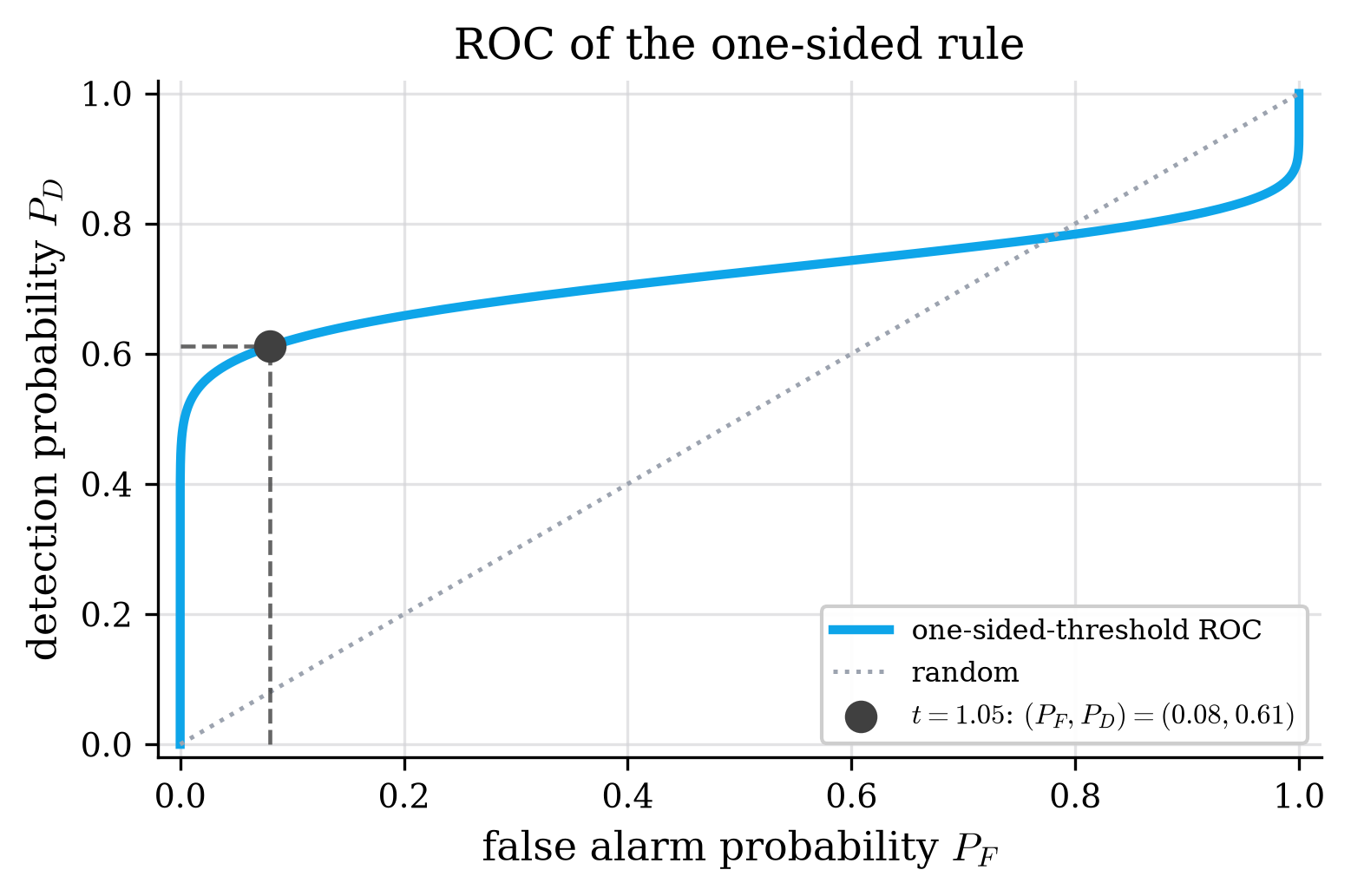
The diagonal is a coin flip. Better separation pushes the curve to the top-left corner.
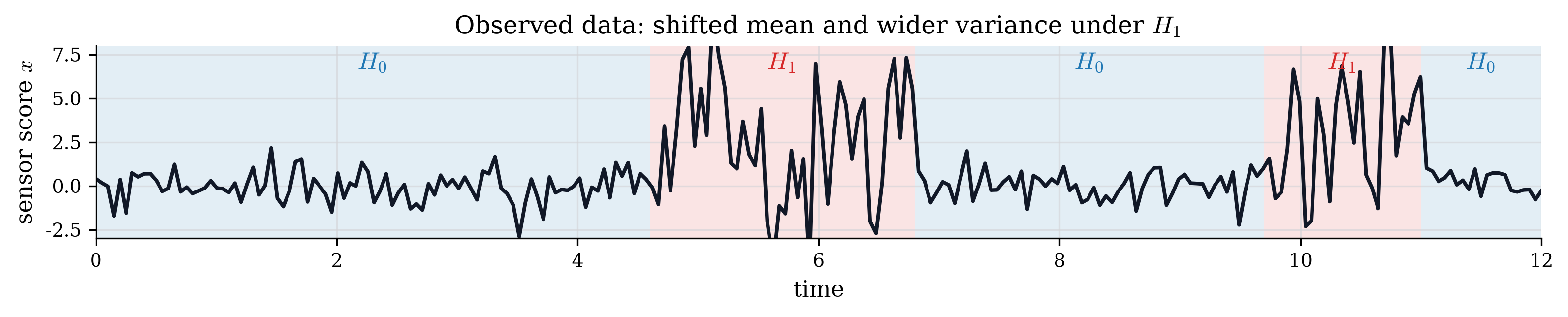
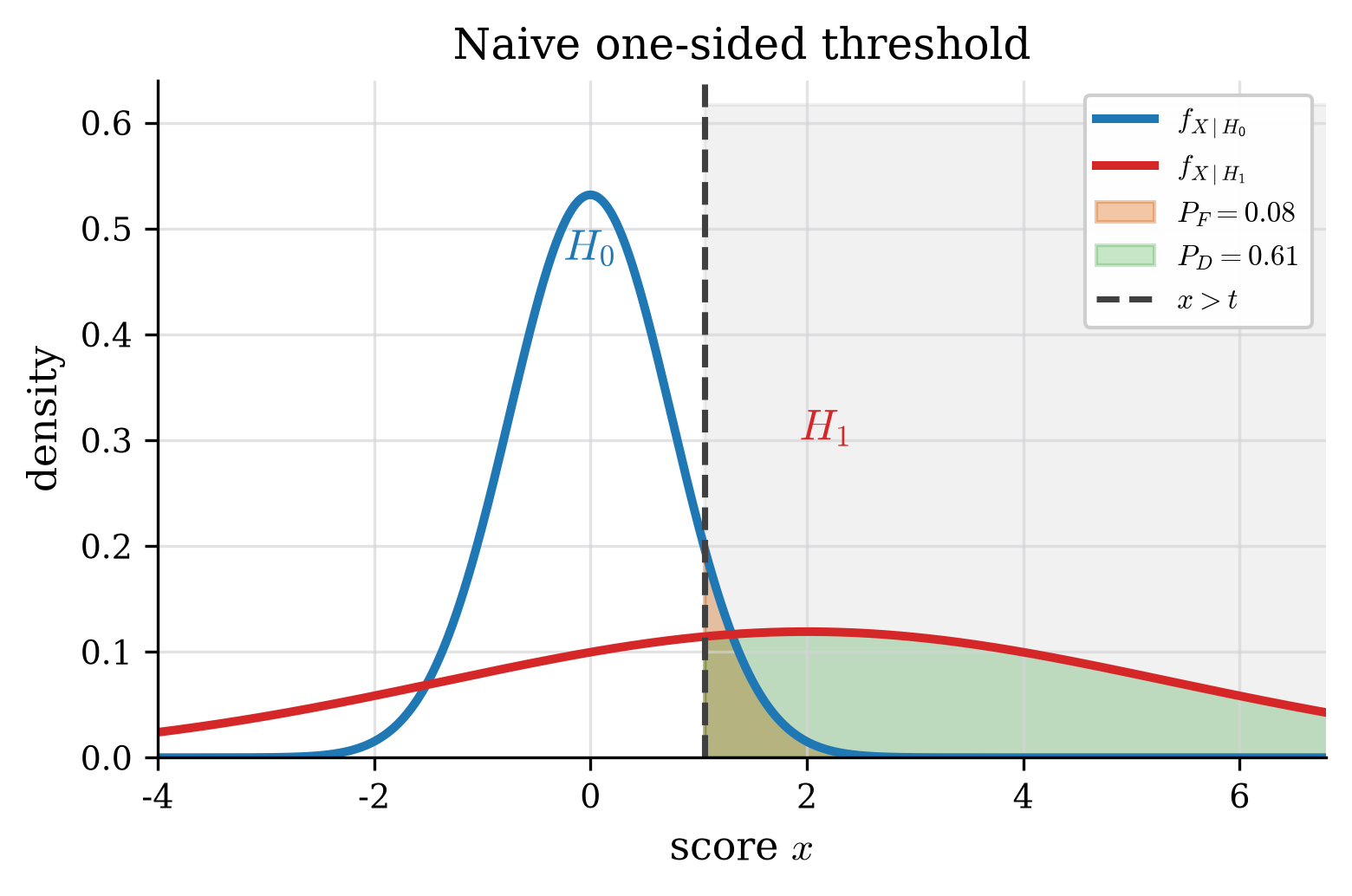
A door sensor reports a score every second. Threshold it, collect the two conditional histograms, sweep the threshold.
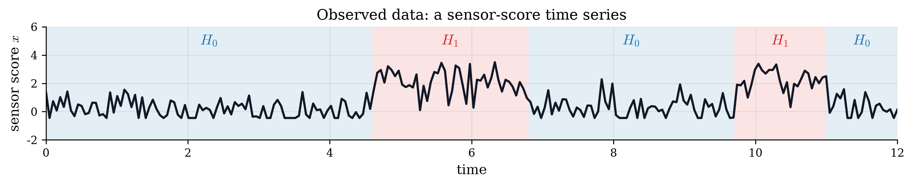
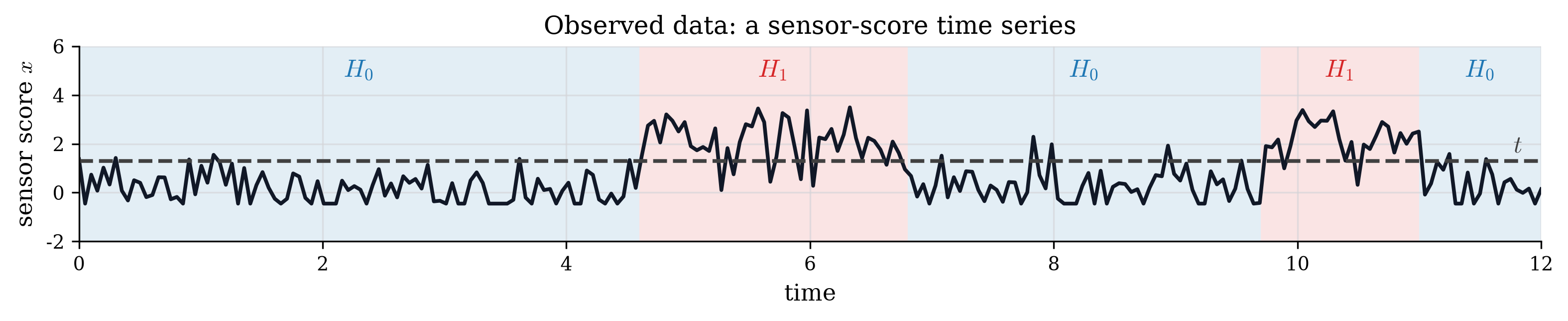
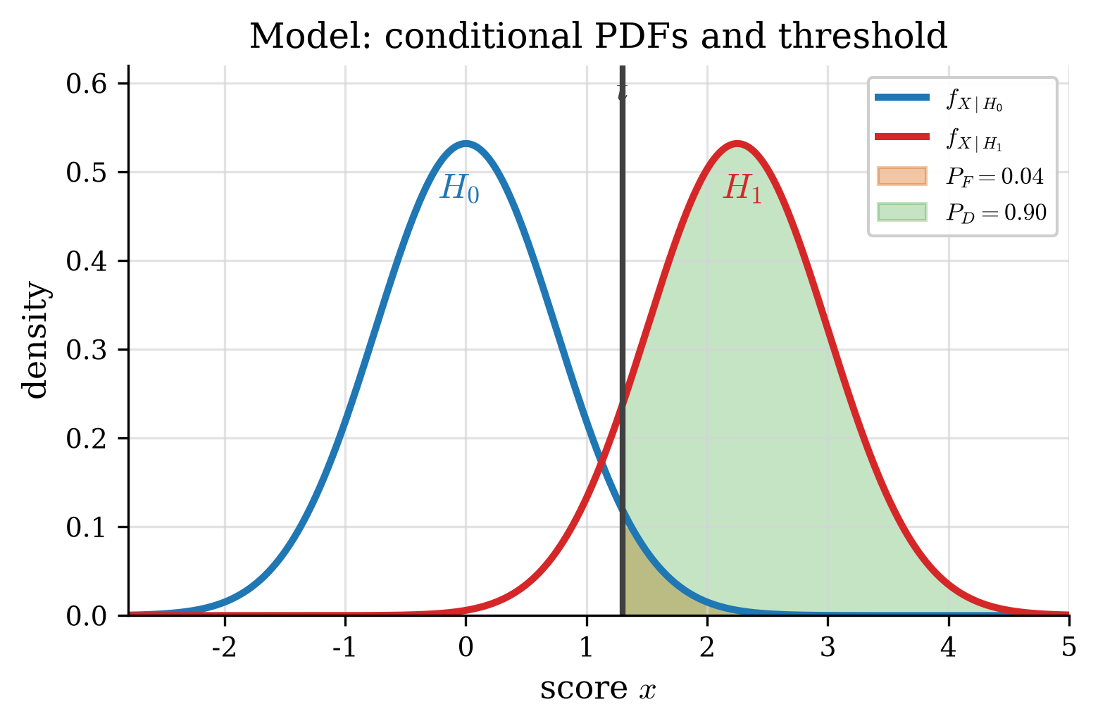
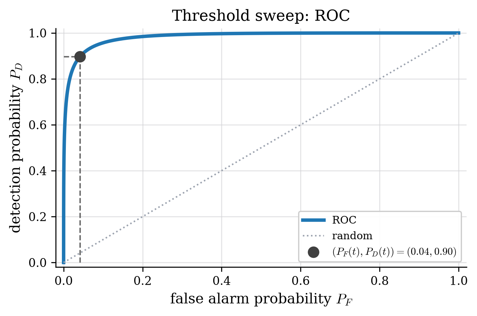

One threshold is one operating point. The curve is the whole family of rules of this form, and choosing a detector means choosing a point on it.


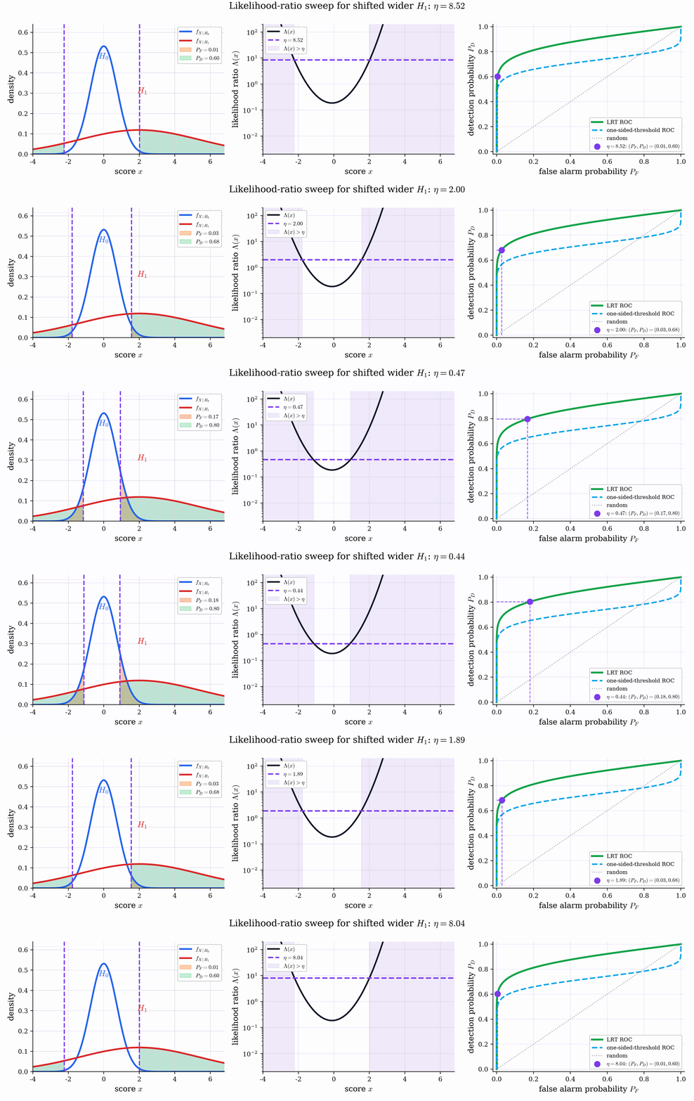
When an intruder changes the spread of the score and not only its level, a threshold on \(x\) is the wrong shape of rule. What should be thresholded?
\[\Lambda(\mathbf x)=\frac{f(\mathbf x;H_1)}{f(\mathbf x;H_0)}\;\underset{H_0}{\overset{H_1}{\gtrless}}\;t\]
Neyman–Pearson lemma Among all rules with false-alarm rate \(P_F\le\alpha\), the likelihood-ratio test maximizes \(P_D\).
Why. \(P_D-t\,P_F=\int_{\mathcal X_1}\bracket{f(\mathbf x;H_1)-t\,f(\mathbf x;H_0)}\dd\mathbf x\) is largest if \(\mathcal X_1\) collects exactly the points where the integrand is positive, which is where \(\Lambda(\mathbf x)>t\). The false-alarm budget fixes \(t\).
The rule is never “compare \(x\) with a number”; it is “compare \(\Lambda(\mathbf x)\) with a number.” The lemma needs simple hypotheses: no unknown parameter left inside either density.

The region \(\set{\Lambda>t}\) is two tails, not an interval: an extreme score either way is what the wide alternative predicts. Its ROC lies above the simple threshold’s everywhere.
A known level in Gaussian noise \(X=\pm A+N\), \(N\sim\Gauss(0,\sigma^2)\). Then \(\ln\Lambda(x)=2Ax/\sigma^2\) is linear in \(x\), so the test is a threshold on \(x\) after all, and \(P_F=Q\!\paren{\tfrac{\gamma+A}{\sigma}}\), \(P_D=Q\!\paren{\tfrac{\gamma-A}{\sigma}}\).
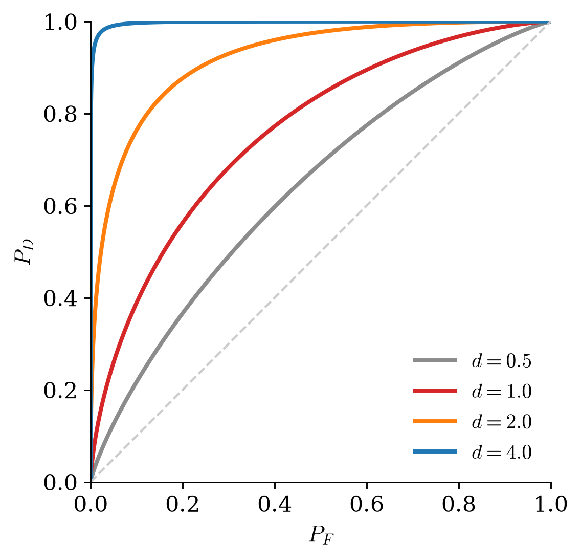
The ROC depends only on \(d=2A/\sigma\), the separation in noise units. That is why detection performance is always quoted as a signal-to-noise ratio.
A classroom experiment Write down a sequence of 30 heads and tails. Half of the room: flip a real coin. The other half: invent the sequence, as randomly as you can. Mark which you did, and hand it in.
While we collect: can we tell the two piles apart, without knowing which is which?
The obvious test: the fraction of heads \(\widehat P_H\). Under \(H_0\) (fair, independent coin) it is a sample mean of \(N\) Bernoulli\((\tfrac12)\) tosses, so \(H_0\) supplies its mean and its variance:
The \(z\)-test \[Z_H=\frac{\widehat P_H-\tfrac12}{1/(2\sqrt{N})}\;\overset{H_0}{\approx}\;\Gauss(0,1), \qquad\text{reject if }\abs{Z_H}>2 .\]
Compute it for both piles. Both pass: people know that a coin shows heads half the time.
Nothing unknown in the null distribution, so this is the \(z\)-test in its exact setting. But a passed test says only that this statistic saw nothing.
Count the steps where the outcome changes. For a fair, independent coin these are \(N-1\) iid Bernoulli\((\tfrac12)\) indicators, so the same test applies with \(N-1\) in place of \(N\): \[Z_A=\frac{\widehat P_A-\tfrac12}{1/(2\sqrt{N-1})} .\]

People break up runs because runs look unrandom, and alternate at about \(0.6\): \(Z_A\approx2\) at \(N=100\). Same formula, a different statistic: real randomness has longer runs than intuition expects.
Hold the data fixed and let the parameter vary: \(f(\mathbf x;\phi)\) becomes the likelihood of \(\phi\). \[\widehat\phi_{\text{ML}}=\argmax_\phi\ \ln f(\mathbf x;\phi) =\argmax_\phi\ \sum_{k=1}^N\ln f_X(x_k;\phi).\]

Detection compared two members of the family. Maximum likelihood compares all of them: \(\widehat\phi_{\text{ML}}\) is the candidate that wins every pairwise likelihood-ratio test at threshold \(t=1\).
The Gaussian mean With \(\sigma^2\) known, \(\ln f=-\frac{1}{2\sigma^2}\sum_k(x_k-\phi)^2+\text{const}\), so \[\frac{\partial}{\partial\phi}\ln f=\frac{1}{\sigma^2}\sum_k(x_k-\phi)=0 \quad\Longrightarrow\quad \widehat\phi_{\text{ML}}=\frac1N\sum_k x_k .\]

The sample mean was maximum likelihood all along, for Gaussian data. The logarithm moved no maximum: it turned the product into a sum, one term per observation.
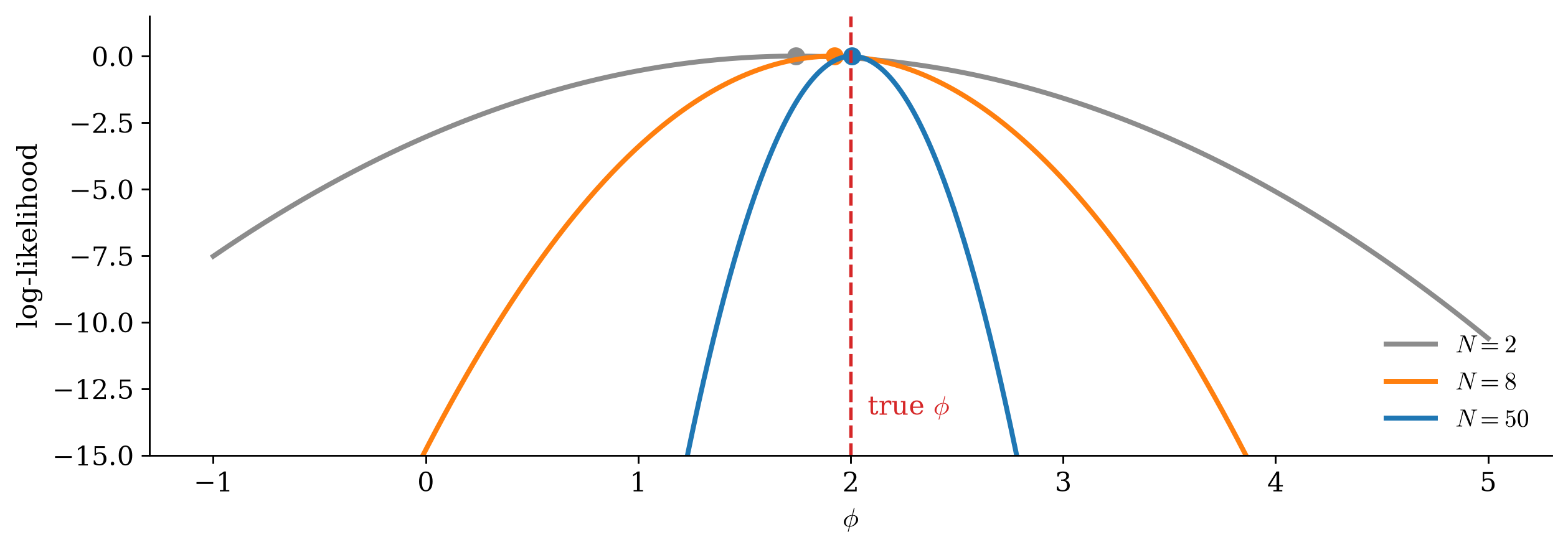
More data barely moves the peak; it makes it sharper. A sharp peak means the data tell nearby values of \(\phi\) apart. The curvature at the peak is the subject of the last part.
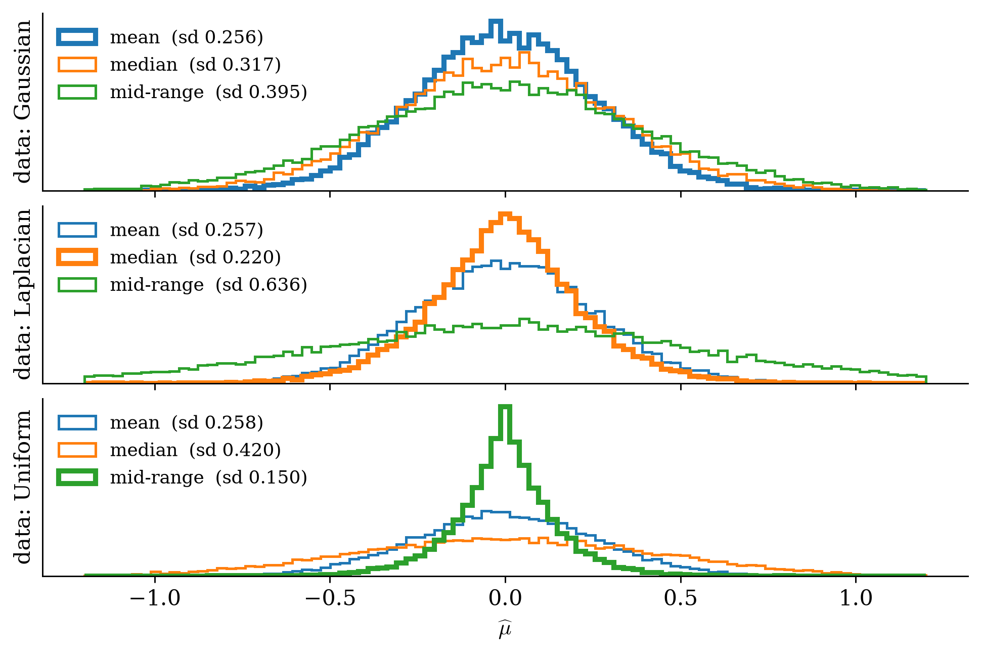
The same unknown in all three: the center \(m\) of a symmetric law. Only the noise model changes.
| noise model | log-likelihood | ML estimate of \(m\) |
|---|---|---|
| Gaussian, known \(\sigma^2\) | \(-\frac{1}{2\sigma^2}\sum_k(x_k-m)^2\) | sample mean \(\bar x\) |
| Laplacian, known \(b\) | \(-\frac1b\sum_k\abs{x_k-m}\) | sample median |
| Uniform on \([m-h,m+h]\), known \(h\) | \(-N\ln(2h)\) if every \(\abs{x_k-m}\le h\) | midrange \(\tfrac12(\min_kx_k+\max_kx_k)\) |
The noise model chooses the loss. One estimator uses every sample, one essentially one (the middle), one exactly two (the extremes), and each is right for its own tails.
Each time stamp has density \(1/\phi\) on \([0,\phi]\), and \(0\) beyond it. So \[f(\mathbf x;\phi)=\begin{cases}\phi^{-N}, & \phi\ge\max_kx_k,\\ 0, & \text{otherwise.}\end{cases}\]
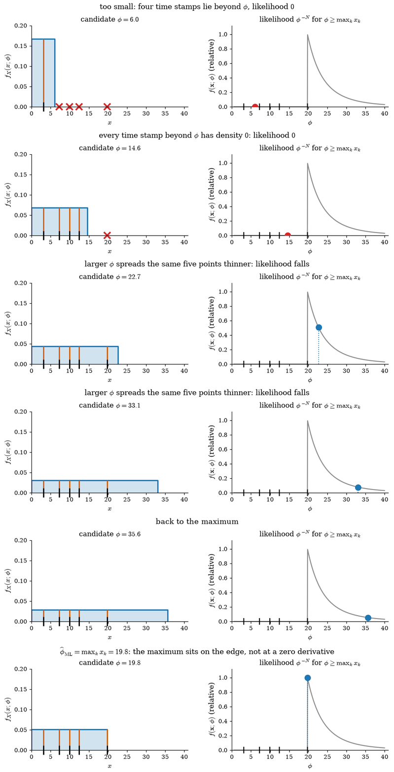
No derivative is zero anywhere: the maximum sits on the edge of the admissible set. Any smaller \(\phi\) rules out a time stamp we saw; any larger one spreads the same five points more thinly.
\(N\) points drop into \([0,\phi]\) and cut it into \(N+1\) gaps. By symmetry the gaps have the same expected length, \(\phi/(N+1)\), including the one between the largest value and the edge.
So the maximum falls short by one gap on average, \(\E{\max_kX_k}=\frac{N}{N+1}\,\phi\), and the fix adds the average gap seen in the data: \[\widehat\phi=\frac{N+1}{N}\max_kx_k=\max_kx_k+\frac{\max_kx_k}{N}=19.8+3.96=23.76 .\]

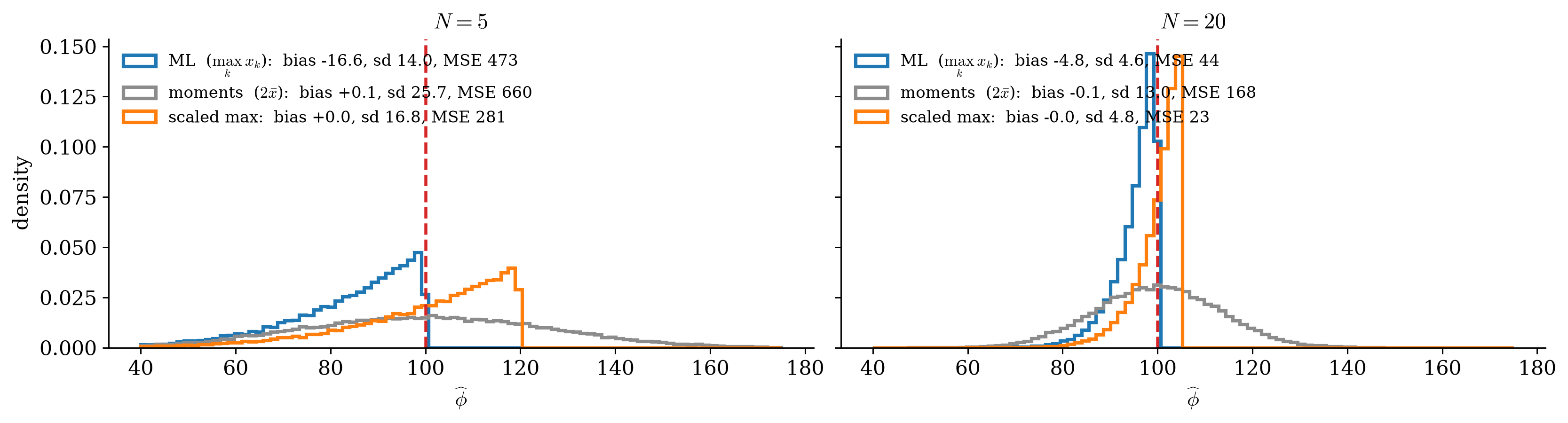
The maximum can never exceed the truth, so ML is biased low, yet it has the smallest spread. Scaling by \((N+1)/N\) removes the bias for a little extra spread. Both leave the moment estimator far behind.
Score and Fisher information \[S(\mathbf X;\phi)=\frac{\partial}{\partial\phi}\ln f(\mathbf X;\phi),\qquad I(\phi)=\E{S(\mathbf X;\phi)^2}.\]
The score is the slope of the log-likelihood at \(\phi\). It has mean zero at the true parameter, and its spread, \(I(\phi)\), measures how sharply the likelihood depends on \(\phi\): the curvature of the likelihood we watched sharpen with \(N\), averaged over the data.
For an iid sample the scores add, and so does the information: \(I_N(\phi)=N\,I_1(\phi)\).
Cramér–Rao bound Every unbiased estimator satisfies \(\Var{\widehat\Phi}\ge 1/I(\phi)\).
Why. The error of an unbiased estimator is correlated with the score (their covariance is exactly \(1\)), and a correlation coefficient cannot exceed one: by Cauchy–Schwarz, \(1\le\Var{\widehat\Phi}\,I(\phi)\).
A floor under every unbiased estimator, however clever, and it falls like \(1/N\).
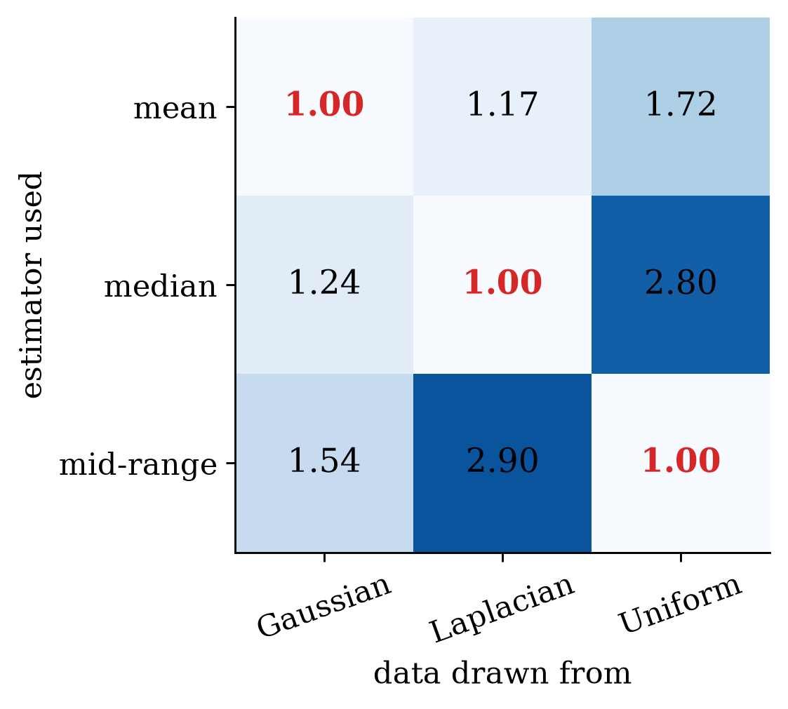
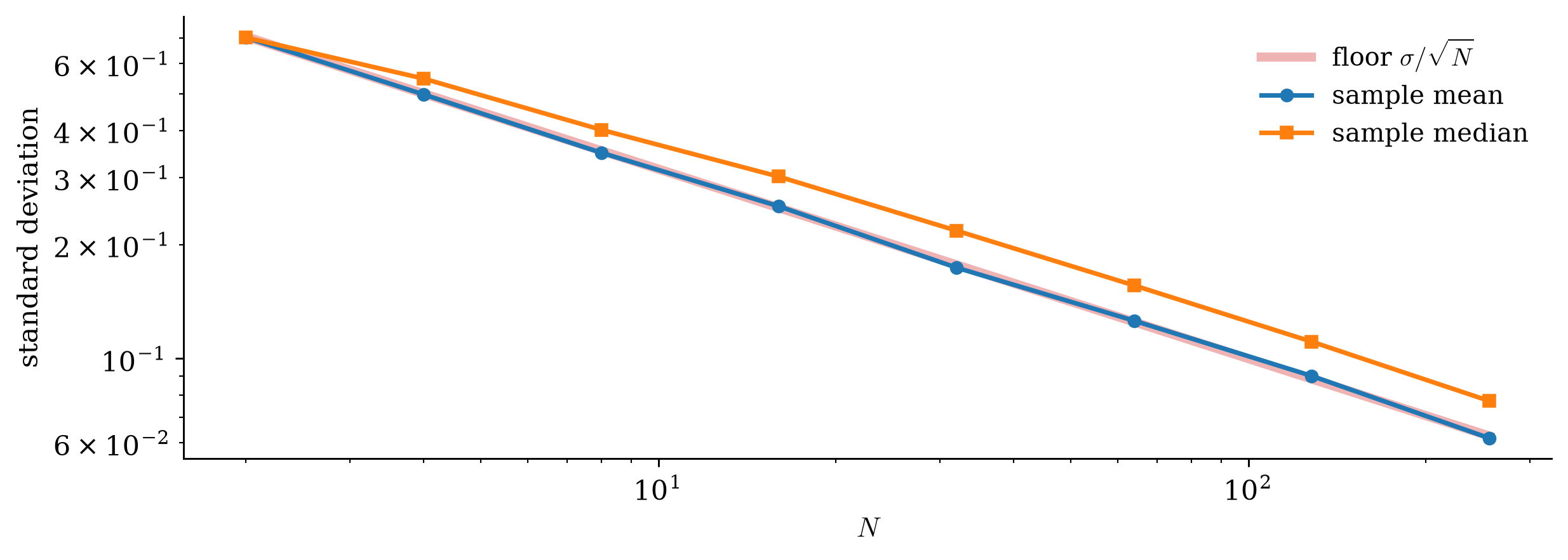
For Gaussian data \(I_N=N/\sigma^2\): no unbiased estimator beats \(\sigma^2/N\), and the sample mean sits exactly on it. The median pays about 25% in spread.
For Gaussian data the information about \(\sigma^2\) is \(I=N/(2\sigma^4)\), so every unbiased estimator of the variance has \(\Var{\widehat\Sigma^2}\ge 2\sigma^4/N\).
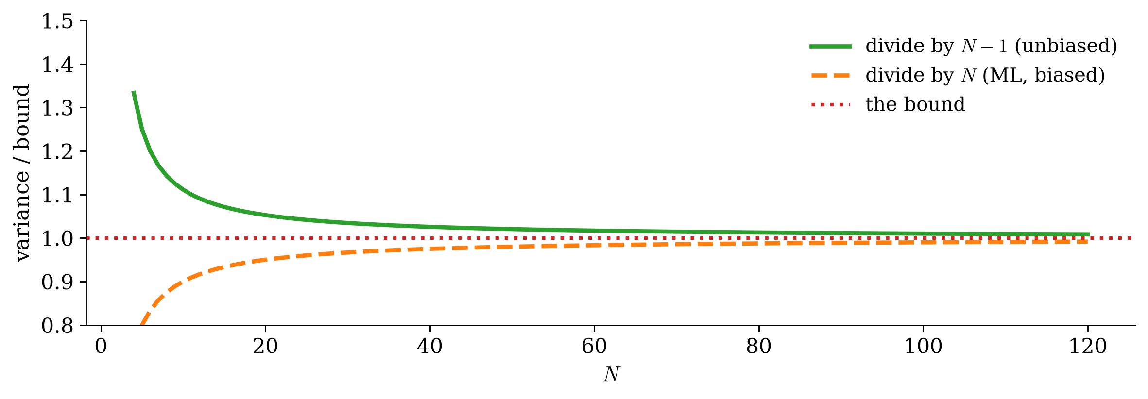
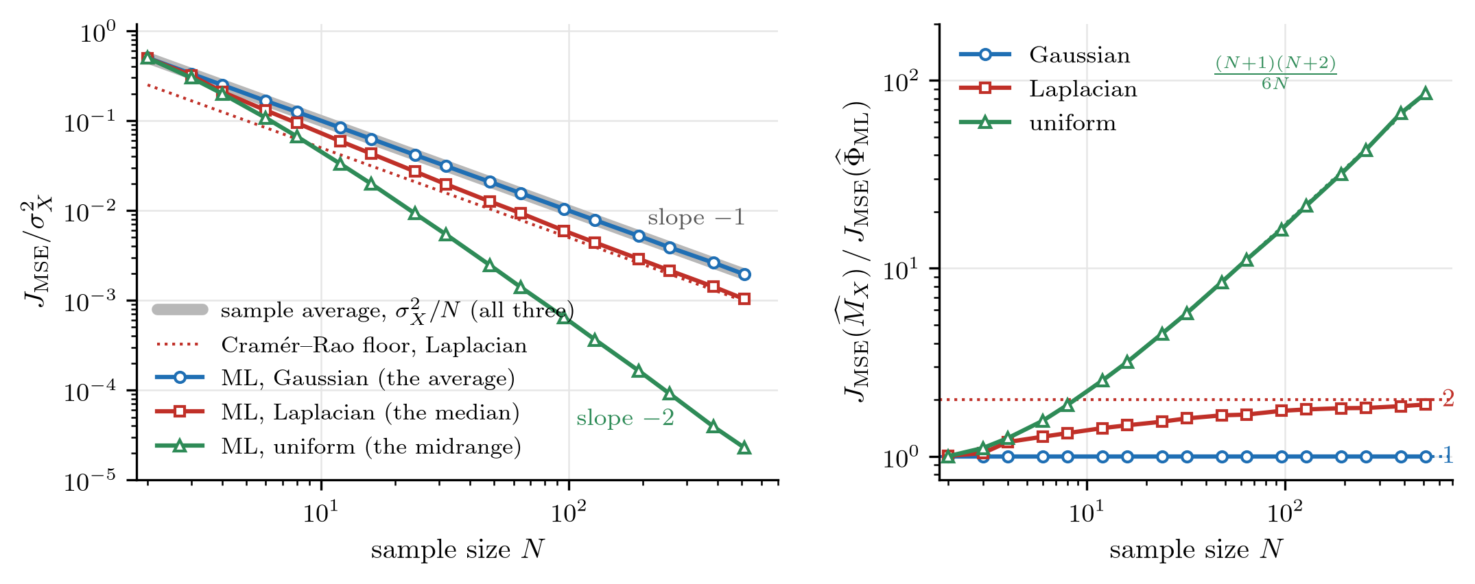
The unbiased estimator never reaches the bound: it is a lower limit, not a promise. The ML curve sits below it, which is no contradiction, since the bound speaks only about unbiased estimators.

The average cannot tell the three laws apart, because it never looks at the density. ML does: it is twice as good for Laplacian data, and for uniform data its error falls like \(1/N^2\) instead of \(1/N\).
Maximum likelihood, as \(N\to\infty\)
All three are asymptotic. None of them says anything about \(N=12\), which is the case you usually have.
The bound assumes the support of \(f_X(x;\phi)\) does not move with \(\phi\). The puzzle breaks exactly that: the data live on \([0,\phi]\), whose edge is the parameter, and the score is the constant \(-N/\phi\), which cannot have mean zero.
The scaled maximum \[\Var{\widehat\Phi}=\frac{\phi^2}{N(N+2)}:\] an error falling like \(1/N\) rather than \(1/\sqrt N\). An edge is located far more precisely than a center.
“The Cramér–Rao bound is the best possible” is a statement about unbiased estimators in regular models. The Gaussian mean is both; the range of a uniform is neither.
| estimator | bias | variance | error falls like |
|---|---|---|---|
| twice the average (moments) | \(0\) | \(\phi^2/(3N)\) | \(1/\sqrt N\) |
| largest value (ML) | \(-\phi/(N+1)\) | \(\approx\phi^2/N^2\) | \(1/N\) |
| scaled maximum | \(0\) | \(\phi^2/(N(N+2))\) | \(1/N\) |
For the five time stamps: \(20.96\), \(19.8\), \(23.76\). Reading only the average threw away the information that sits at the edge, and no amount of cleverness with the average recovers it.
This week