One Formula, Four Instruments

Matched filter, beamformer, regularized inverse, fusion

Four jobs

\[ % Number sets \newcommand{\Nat}{\mathbb{N}} \newcommand{\Integer}{\mathbb{Z}} \newcommand{\Real}{\mathbb{R}} \newcommand{\Complex}{\mathbb{C}} % Operators \newcommand{\SNR}{\operatorname{SNR}} \newcommand{\tr}{\operatorname{tr}} \newcommand{\re}{\operatorname{Re}} \newcommand{\im}{\operatorname{Im}} \newcommand{\sign}{\operatorname{sign}} \newcommand{\rect}{\operatorname{rect}} \newcommand{\sinc}{\operatorname{si}} \newcommand{\erf}{\operatorname{erf}} \newcommand{\erfc}{\operatorname{erfc}} \newcommand{\kurt}{\operatorname{kurt}} \newcommand{\diag}{\operatorname{diag}} \newcommand{\MSE}{\operatorname{MSE}} \newcommand{\argmin}{\operatorname*{argmin}} \newcommand{\argmax}{\operatorname*{argmax}} \newcommand{\bias}{\operatorname{bias}} \newcommand{\Bin}{\operatorname{Bin}} % Delimiters \newcommand{\paren}[1]{\left(#1\right)} \newcommand{\bracket}[1]{\left[#1\right]} \newcommand{\set}[1]{\left\{#1\right\}} \newcommand{\abs}[1]{\left\lvert #1 \right\rvert} \newcommand{\norm}[1]{\left\lVert #1 \right\rVert} \newcommand{\ip}[1]{\left\langle #1 \right\rangle} % Notation \newcommand{\dd}{\,\mathrm{d}} \newcommand{\tran}{^{\top}} \newcommand{\conv}{\ast} \newcommand{\conj}{^{*}} \newcommand{\herm}{^{\mathsf{H}}} \newcommand{\opt}{^{\star}} % Expectation and variance % \newcommand{\E}[1]{\mathbb{E}\!\left[#1\right]} \newcommand{\E}[2][]{\mathbb{E}_{#1}\!\left[#2\right]} \newcommand{\Var}[1]{\mathbb{V}\!\left[#1\right]} % Distributions \newcommand{\Gauss}{\mathcal{N}} \newcommand{\Uniform}{\mathcal{U}} \newcommand{\FT}{\mathcal{F}} % Probability \newcommand{\Prob}[1]{\mathbb{P}\!\left(#1\right)} % Misc \newcommand{\bsy}[1]{\boldsymbol{#1}} \newcommand{\calR}{\mathcal{R}} \newcommand{\calC}{\mathcal{C}} \]

Four instruments, one idea

• Radar. Is a known pulse buried in this noisy echo?
• Microphone array. Listen to one talker and suppress the one next to them.
• Spectrometer. Which substances, in what amounts, produced this blurred mixture?
• Navigation. Combine a satellite fix with an inertial sensor that measures something else.

One answer Each has a known signature (a template, a steering vector, a forward model, a measurement map) and noise with a known covariance, and each answer has the same form: \[\mathbf R^{-1}\times\text{the known signature}.\]

In the notes The Matched Filter · Multichannel Estimation and Beamforming · Inverse Problems · Sensor Fusion

This week has no new theory. It is the projection of estimation-as-projection and the whitening of the random-vector week, applied four times. The point to land is the common form of the four answers.

A notation for who knows what

The marks used in every signal-flow figure: each symbol carries one mark saying whether it is known, random, observed, or sought.

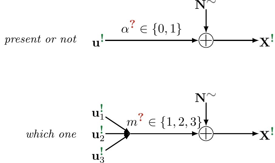
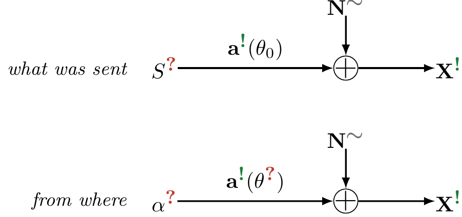
The four instruments differ only in where the question mark sits: on the arrow (is the template there?), on the direction (where is the source?), on the cause (what produced this?), on the state seen by several sensors.

The matched filter

Is the template there?

Detecting a known template \[H_0:\ \mathbf X=\mathbf N\qquad\text{vs.}\qquad H_1:\ \mathbf X=\mathbf u+\mathbf N,\] with \(\mathbf u\) a known template and \(\mathbf N\) zero-mean noise of covariance \(\mathbf R_{\mathbf{NN}}\).

Is the template there?

Detection as a signal flow: the template known, the noise random, and the question mark on the arrow.

Two roads to a detector: assume a distribution and ask for the optimal test, or assume nothing and ask for the best linear score.

Road 1: the Gaussian likelihood ratio

With Gaussian noise both hypotheses give Gaussian data differing only in the mean, so the quadratic terms cancel in the log-likelihood ratio:

Gaussian log-likelihood ratio \[\ln\Lambda(\mathbf x)=\re\set{\mathbf u\herm\mathbf R_{\mathbf{NN}}^{-1}\mathbf x}-\tfrac12\,\mathbf u\herm\mathbf R_{\mathbf{NN}}^{-1}\mathbf u .\]

The Neyman–Pearson test, optimal among all tests, thresholds a statistic linear in the data, with weights \(\mathbf R_{\mathbf{NN}}^{-1}\mathbf u\).

For a Gaussian signal-in-noise problem the optimal detector simply is a linear filter. Nothing forced that; it fell out of the cancellation.

Road 2: the best linear score

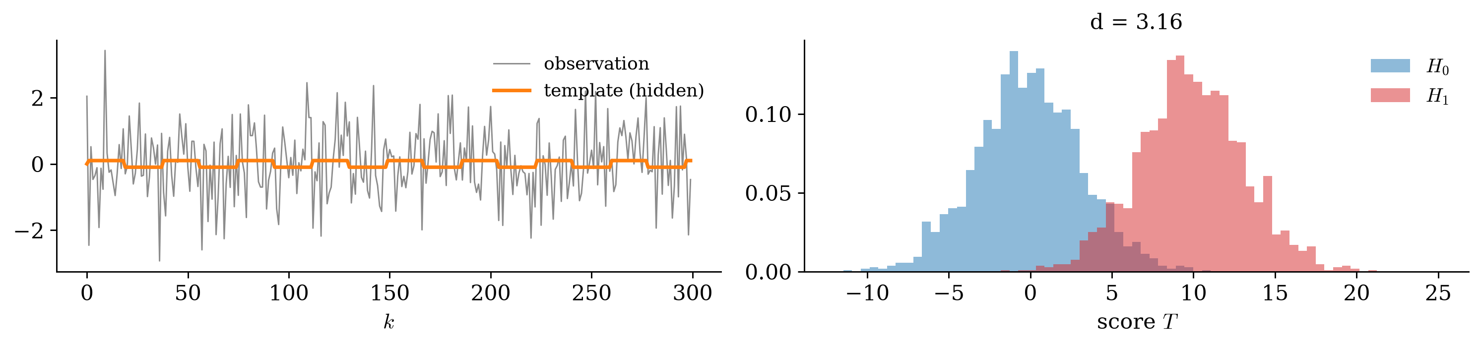
Assume nothing about the distribution. Score with \(T=\mathbf w\herm\mathbf X\) and ask for the largest separation of the hypotheses in noise units, the deflection: \[d^2(\mathbf w)=\frac{\abs{\E{T\mid H_1}-\E{T\mid H_0}}^2}{\Var{T\mid H_0}} =\frac{\abs{\mathbf w\herm\mathbf u}^2}{\mathbf w\herm\mathbf R_{\mathbf{NN}}\mathbf w}.\]

Matched filter \[\mathbf w\opt\propto\mathbf R_{\mathbf{NN}}^{-1}\mathbf u,\qquad d^2_{\max}=\mathbf u\herm\mathbf R_{\mathbf{NN}}^{-1}\mathbf u .\]

Whiten, then Cauchy–Schwarz

Proof Substitute \(\mathbf a=\mathbf R_{\mathbf{NN}}^{1/2}\mathbf w\) and \(\mathbf b=\mathbf R_{\mathbf{NN}}^{-1/2}\mathbf u\): the noise becomes white, and \[d^2=\frac{\abs{\mathbf a\herm\mathbf b}^2}{\norm{\mathbf a}^2}\le\norm{\mathbf b}^2=\mathbf u\herm\mathbf R_{\mathbf{NN}}^{-1}\mathbf u,\] with equality when \(\mathbf a\parallel\mathbf b\).

Only the direction of \(\mathbf w\) matters; the scale is absorbed by the threshold.

The proof is the two tools of the random-vector week, in order: whiten, then measure an angle.

Where the two roads meet, and where they part

Two roads

• Gaussian noise: they agree. The log-likelihood ratio was already linear, so the best linear score is the best test.

• Otherwise: they separate. The matched filter still maximizes deflection, but the optimal detector is some nonlinear function of the data.

The same pattern as the Gaussian estimation theorem, one criterion over: Gaussianity is what collapses “best linear” into “best”, in detection exactly as in estimation.

In white noise: just correlate

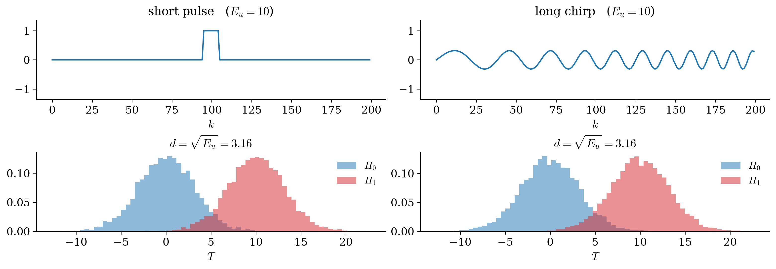
With \(\mathbf R_{\mathbf{NN}}=R_0\mathbf I\) the weights are the template: \[T=\frac{1}{R_0}\ip{\mathbf X,\mathbf u},\qquad d^2_{\max}=\frac{E_u}{R_0},\qquad E_u=\norm{\mathbf u}^2 .\]

A known pulse in noise: correlating with the template and thresholding the score is the Neyman–Pearson test.

→ Demo: matched filter detection

Processing gain

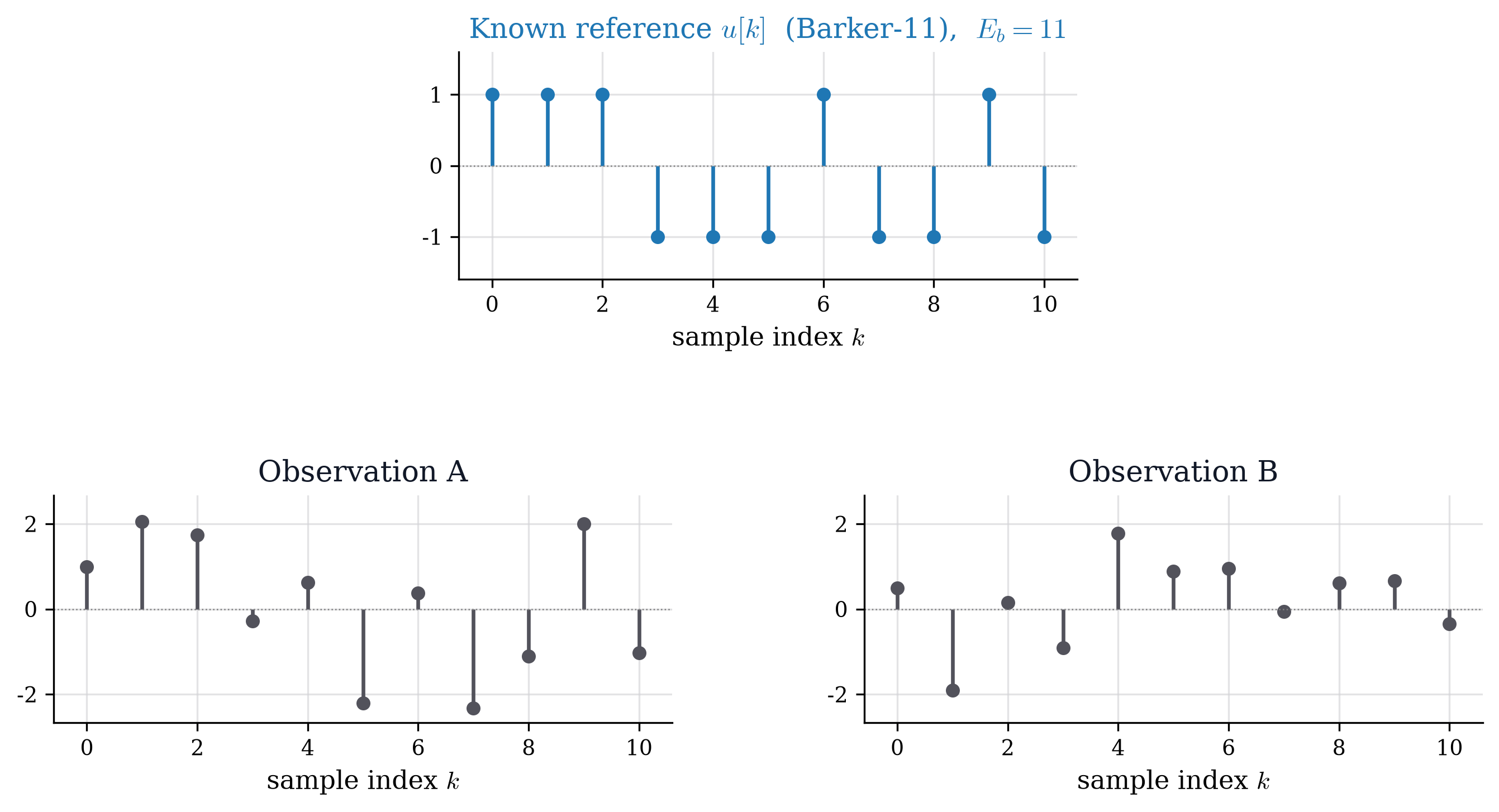
In white noise with per-sample signal-to-noise ratio \(\text{SNR}_1=\abs{u}^2/R_0\) over \(N\) samples, \[d^2_{\max}=\frac{E_u}{R_0}=N\cdot\text{SNR}_1 .\]

A template of \(N=1000\) samples at \(-20\) dB per sample reaches \(d^2=10\), that is \(+10\) dB: invisible in every sample, obvious in the score.

Figure 1: A 1000-sample template at −20 dB per-sample SNR, hidden in noise (left), and the matched-filter score over 2000 trials with and without it (right).

Energy, not shape

Figure 2: Two templates of identical energy and different shape, and the score under each hypothesis in white noise.

In white noise only the template’s energy matters. That is why radar can spread a pulse over a long quiet chirp, and why spread-spectrum signals can hide below the noise floor in every sample.

In colored noise, shape matters again

Figure 3: Deflection d² = uᴴR⁻¹u for templates of unit energy pointing along each eigenvector of a colored noise covariance.

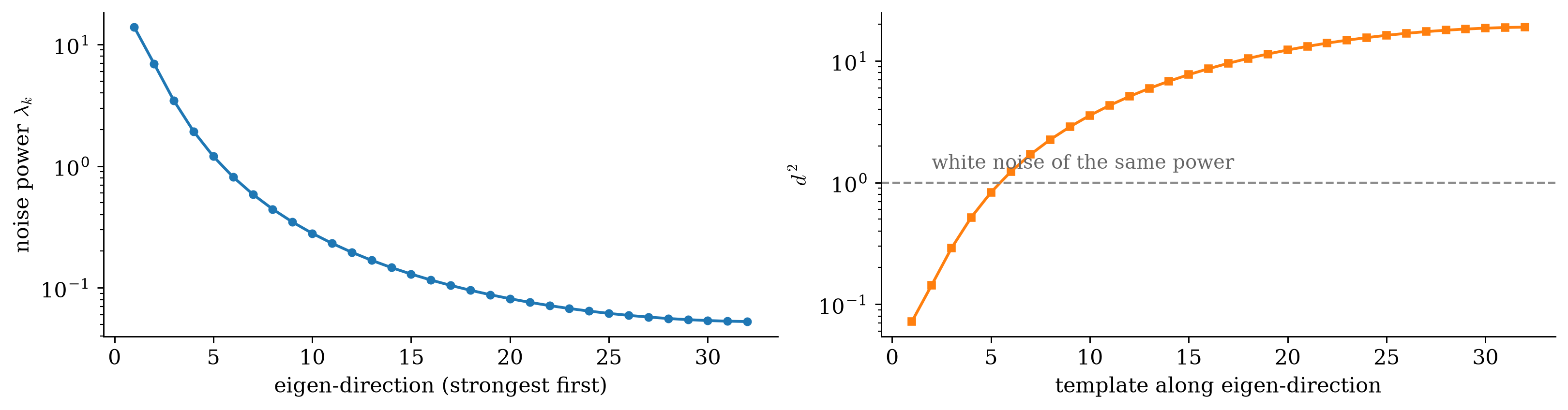
For fixed energy the best template points along the weakest noise eigenvector: put the signal where the noise is not. The same noise that swamps a template in its strong directions is harmless in its weak ones.

The template need not live in time

Detecting one face. Top: the template and four observations of equal energy. Bottom: the score, displaced by the correlation coefficient times the deflection; the ROCs; the template scored against all 400 portraits.

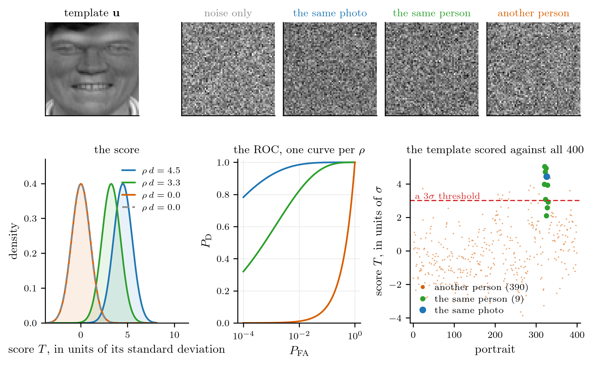
A different photograph of the same person scores lower than the template itself, and a stranger lands on the noise-only curve: the score measures the angle between observation and template.

The beamformer

A direction is a vector

A plane wave from direction \(\theta_0\) reaches each sensor with its own delay.

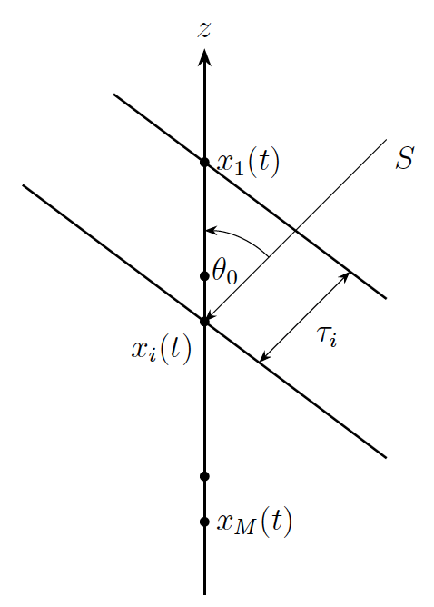
For a narrowband signal the delays are phases: \[\mathbf X=\mathbf a(\theta)\,S+\mathbf N,\qquad[\mathbf a(\theta)]_m=e^{-j\Omega\tau_m(\theta)} .\]

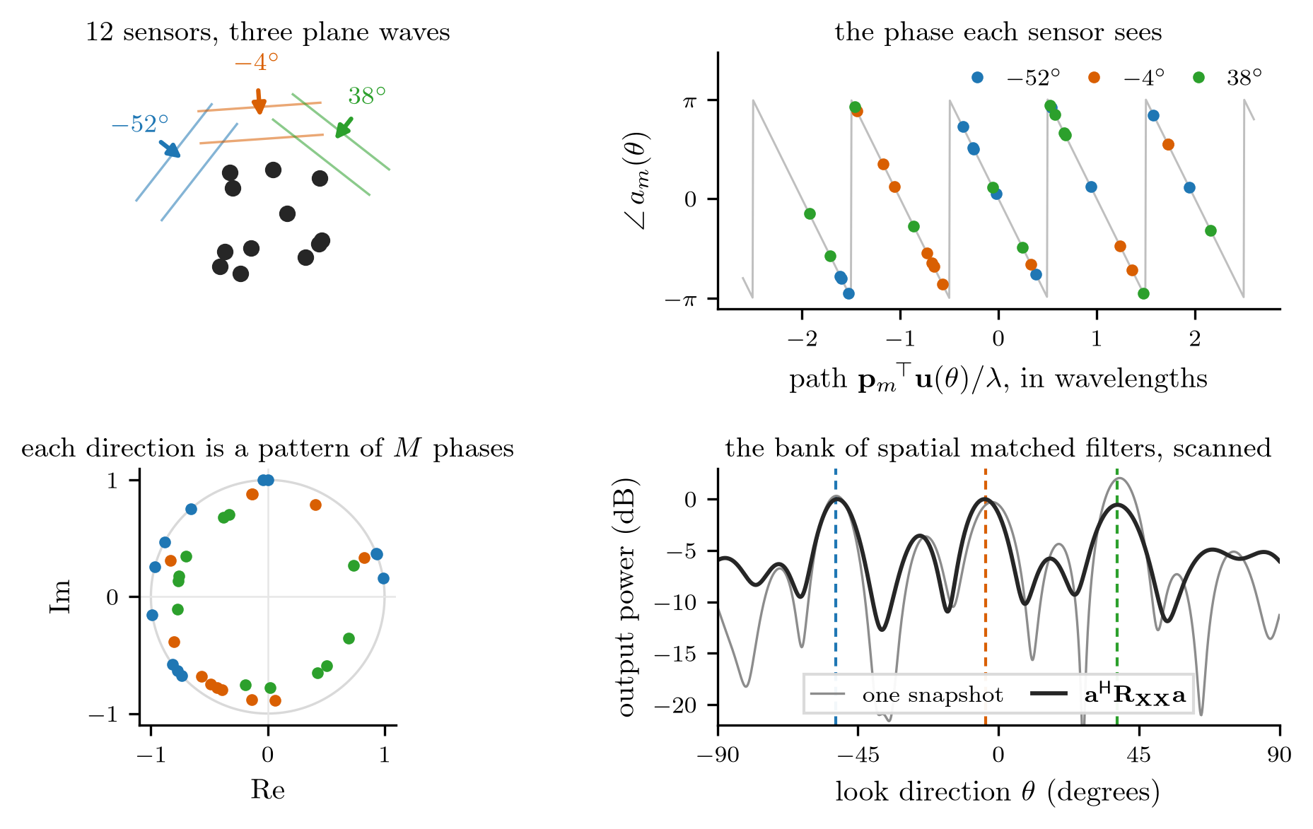
The steering vector is the array’s signature for a direction: no amplitude, only the pattern of relative phases a source there imprints across the aperture.

A direction is a vector

The array as a signal flow. Above, the direction is known and the waveform sought. Below, the question mark moves inside the steering vector.

One model, two questions: what was sent is the beamformer, from where is direction finding.

Steering vectors of a real scene

Twelve sensors at random positions and three plane waves; the phase of each steering vector entry against the extra path; the three steering vectors on the unit circle; and the scan \(\mathbf a(\theta)\herm\mathbf R_{\mathbf{XX}}\mathbf a(\theta)\).

Aperture sets the beam width

Figure 4: Delay-and-sum beampatterns of half-wavelength arrays with 4, 8 and 16 sensors, steered to 0°.

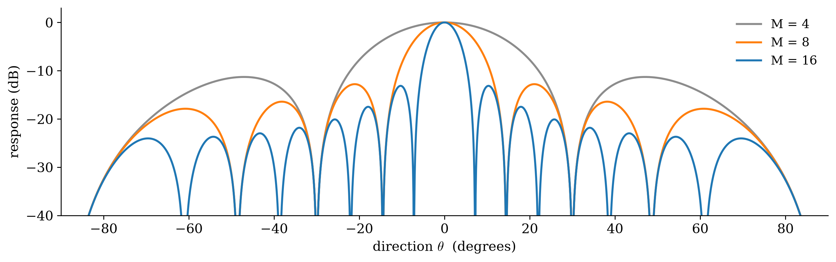
Delay-and-sum is the matched filter for a direction in white noise. Its main lobe narrows like \(1/M\): two sources closer than about one beam width look like one. Resolution is bought with aperture, or with a better covariance model.

Where is the source? A bank of matched filters

One source in proper complex Gaussian noise, \(\mathbf x=\alpha\,\mathbf a(\theta)+\mathbf n\). At each candidate angle, fit the unknown amplitude and compare the likelihoods:

Maximum-likelihood direction \[P(\theta)=\frac{\abs{\mathbf a(\theta)\herm\mathbf R_{\mathbf{NN}}^{-1}\mathbf x}^2}{\mathbf a(\theta)\herm\mathbf R_{\mathbf{NN}}^{-1}\mathbf a(\theta)},\qquad \widehat\theta=\argmax_\theta P(\theta).\]

For every direction: whiten, correlate with its steering vector, normalize. In white noise this is the conventional (Bartlett) scan \(\abs{\mathbf a(\theta)\herm\mathbf x}^2\).

Detection thresholds one matched filter. Parameter estimation runs a family of matched filters and returns the argmax.

Minimum variance, distortionless

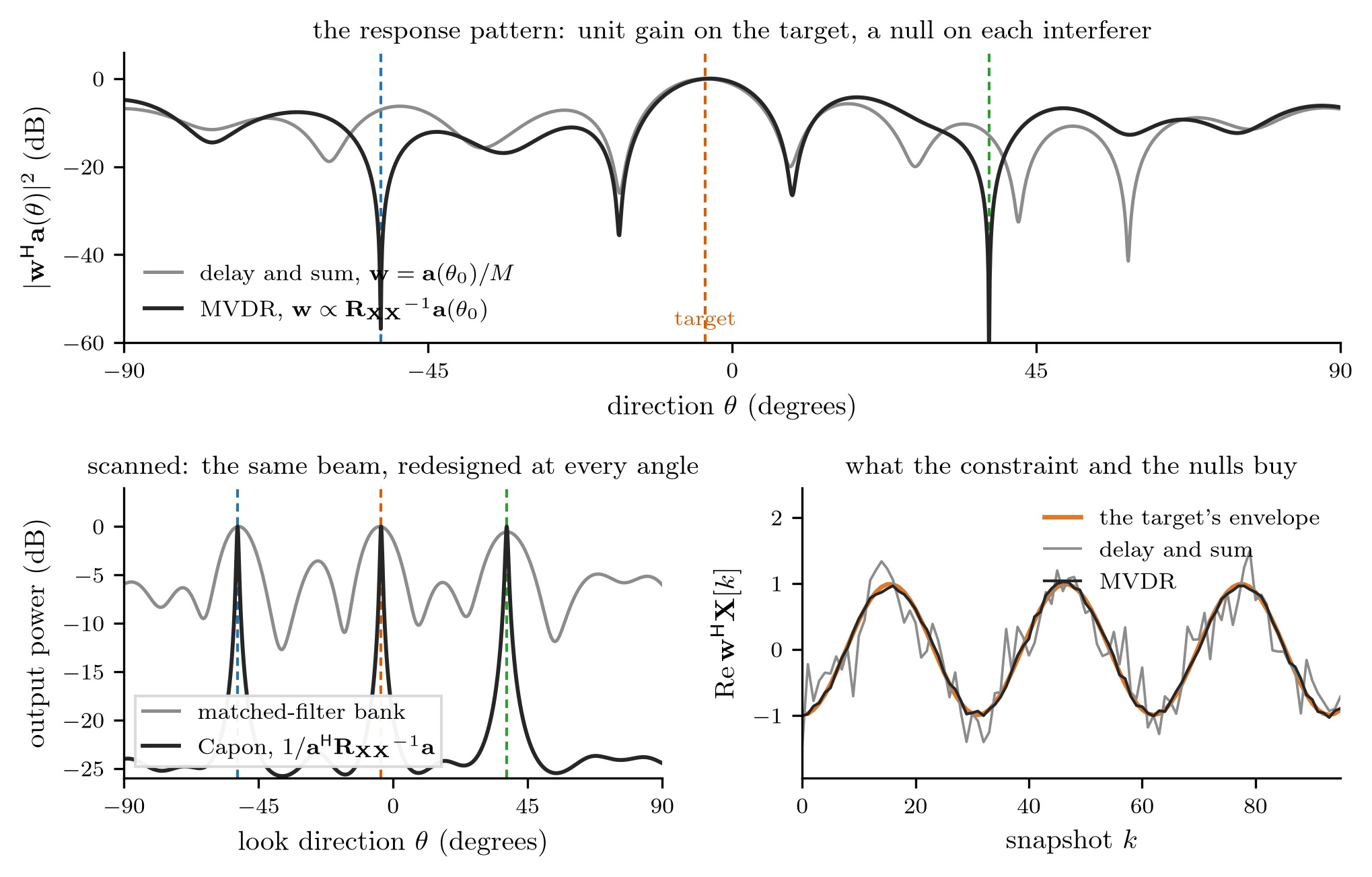
No clean reference signal exists: the array hears every source at once. Replace the reference by a constraint: pass the look direction with gain one, and make everything else as quiet as possible, \[\min_{\mathbf w}\ \mathbf w\herm\mathbf R_{\mathbf{XX}}\mathbf w\quad\text{subject to}\quad\mathbf w\herm\mathbf a(\theta_0)=1 .\]

MVDR beamformer \[\mathbf w_{\text{MVDR}}=\frac{\mathbf R_{\mathbf{XX}}^{-1}\mathbf a(\theta_0)}{\mathbf a(\theta_0)\herm\mathbf R_{\mathbf{XX}}^{-1}\mathbf a(\theta_0)},\qquad P_{\min}(\theta_0)=\frac{1}{\mathbf a(\theta_0)\herm\mathbf R_{\mathbf{XX}}^{-1}\mathbf a(\theta_0)} .\]

The proof is again whiten, then Cauchy–Schwarz. Scanning \(P_{\min}(\theta)\) over directions is the Capon spectrum.

A null nobody asked for

Figure 5: An 8-element array steered to 0°, with a strong interferer at −21°. MVDR was told only the look direction.

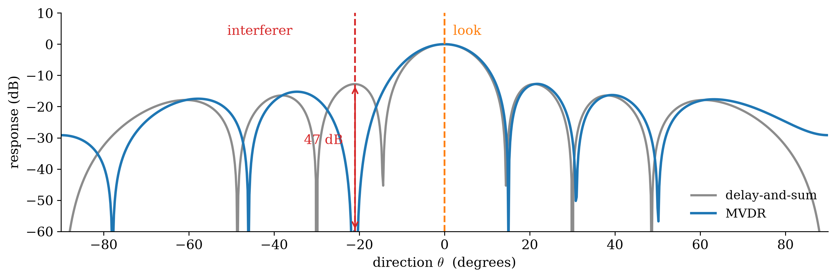
MVDR whitens against \(\mathbf R_{\mathbf{XX}}\), the covariance of the received data including the interference. An interferer inflates \(\mathbf R_{\mathbf{XX}}\) along its own steering vector, and \(\mathbf R_{\mathbf{XX}}^{-1}\) suppresses exactly there.

MVDR on the scene

MVDR on the three-source scene, the middle source as target. Top: its response pattern against delay-and-sum. Bottom left: the Capon spectrum against the matched-filter scan. Bottom right: the target’s envelope and what each beamformer delivers.

→ Demo: delay-and-sum against MVDR, and what a short record does

Several constraints

Pass this direction, null that one: \(\mathbf C\herm\mathbf w=\mathbf g\).

LCMV beamformer \[\mathbf w_{\text{LCMV}}=\mathbf R_{\mathbf{XX}}^{-1}\mathbf C\paren{\mathbf C\herm\mathbf R_{\mathbf{XX}}^{-1}\mathbf C}^{-1}\mathbf g .\]

Each constraint is enforced exactly and costs one of the \(M\) spatial degrees of freedom; what is left fights noise and interference. With one constraint, \(\mathbf C=\mathbf a(\theta_0)\) and \(\mathbf g=1\), this is MVDR again.

The inverse problem

Backwards through a known model

A cause \(\mathbf X\) produces an effect through a known forward operator: \[\mathbf Y=\mathbf A\mathbf X+\mathbf N\qquad(\text{a blur, a mixture, a channel, a projection}).\]

The forward model as a signal flow: operator known, noise random, effect observed, and the cause at the tail of the arrow sought.

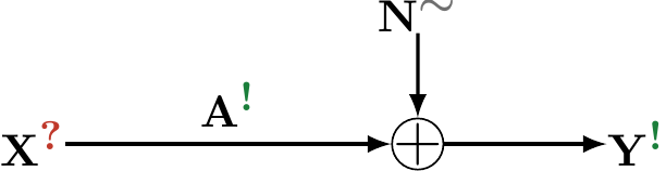
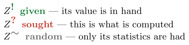
Inverse-problem letters: here the data are \(\mathbf Y\) and the cause \(\mathbf X\) is sought; the marks on the flow say which is which.

The calibrated force/torque sensor is the simplest case: once \(\mathbf A_0\) has been identified, reading an unknown load is this problem with \(\mathbf A=\mathbf A_0\) square and well conditioned.

One model, many problems

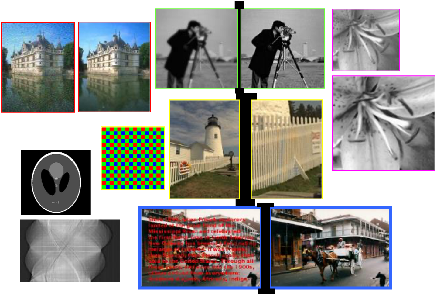
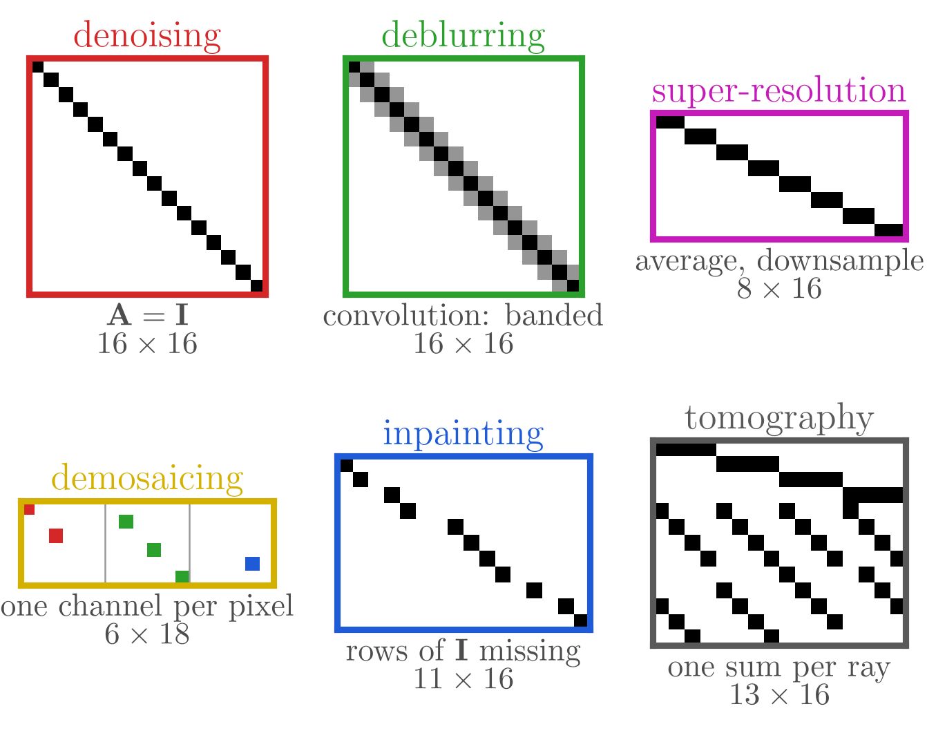
Denoising, deblurring, super-resolution, demosaicing, inpainting, tomography: one \(\mathbf A\) each, one row per measurement. Its shape counts the measurements; its pattern says what each one sees.

When it is easy, and when it is not

If \(\mathbf A\) is tall and full rank the problem is well posed:

Weighted least squares \[\widehat{\mathbf X}=(\mathbf A\herm\mathbf R_{\mathbf{NN}}^{-1}\mathbf A)^{-1}\mathbf A\herm\mathbf R_{\mathbf{NN}}^{-1}\mathbf Y .\]

Most inverse problems are ill posed: \(\mathbf A\herm\mathbf A\) is singular or nearly so. Too few measurements, or directions the operator barely sees.

Inverting then amplifies noise along the weak eigen-directions: the small-eigenvalue blow-up of least squares, in a new costume.

Ill-posed, in the singular values

Figure 6: Singular values of a Gaussian blur on 200 samples, against the noise level of the data.

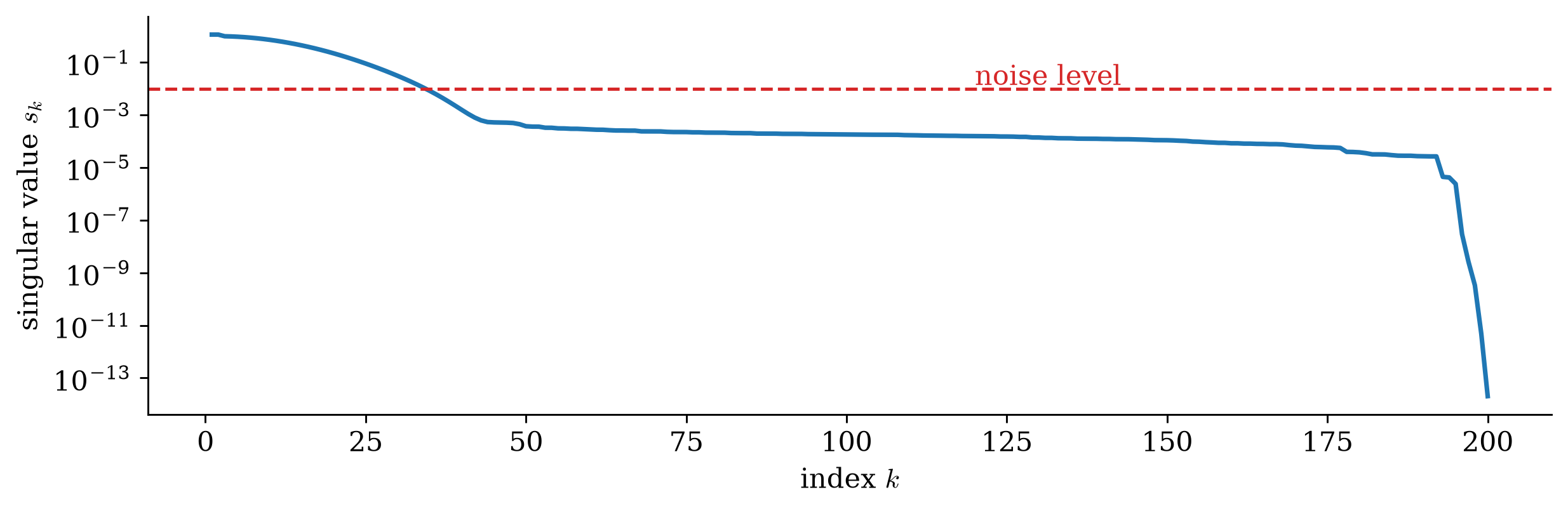
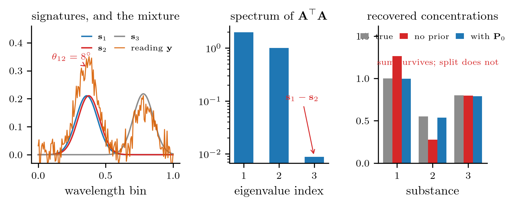
Inverting divides each component by \(s_k\). Below the red line the operator has passed less signal than the noise contains, and dividing by \(s_k\) turns that noise into the answer.

What that looks like

Figure 7: A signal seen through a blur with 1% noise. Naive inversion is worse than doing nothing; the same inversion with a prior recovers the signal.

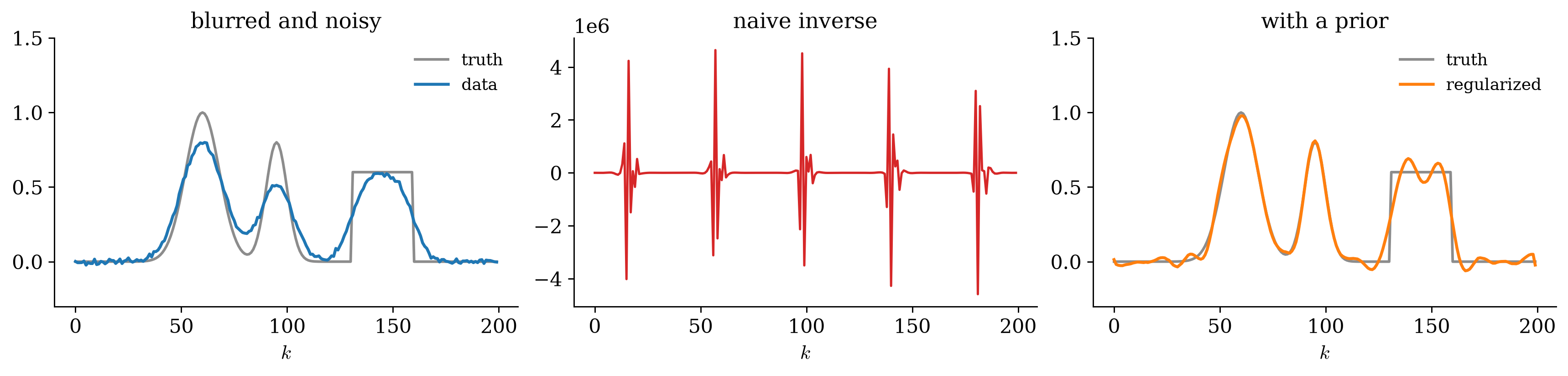
The naive inverse is off the scale. The blur suppressed the signal in some directions, and the inverse faithfully amplifies what is left there, which is noise.

The cure is a prior

Give the cause a prior \((\mathbf m_0,\mathbf P_0)\) and project, exactly as in estimation-as-projection:

Regularized inverse \[\widehat{\mathbf X}=\argmin_{\mathbf x}\ \norm{\mathbf Y-\mathbf A\mathbf x}^2_{\mathbf R_{\mathbf{NN}}^{-1}}+\norm{\mathbf x-\mathbf m_0}^2_{\mathbf P_0^{-1}} =\mathbf m_0+\mathbf P_0\mathbf A\herm\paren{\mathbf A\mathbf P_0\mathbf A\herm+\mathbf R_{\mathbf{NN}}}^{-1}(\mathbf Y-\mathbf A\mathbf m_0).\]

With \(\mathbf m_0=\mathbf 0\), \(\mathbf P_0=\delta^{-1}\mathbf I\), \(\mathbf R_{\mathbf{NN}}=\mathbf I\) it is ridge regression, \((\mathbf A\herm\mathbf A+\delta\mathbf I)^{-1}\mathbf A\herm\mathbf Y\).

The prior covariance, encoding expected size, smoothness or correlation of the unknown, is what lifts the weak directions. Choosing it well is the whole art.

One formula, three claims

Three readings of the regularized inverse

• Penalized least squares: fit the data, penalize implausible \(\mathbf x\). Nothing probabilistic; the inverse covariances are weighting metrics.

• Best linear estimator: needs only the first two moments; gives up global optimality.

• MAP: requires Gaussian noise and a Gaussian prior.

Under joint Gaussianity all three coincide and the answer is optimal among all estimators. Away from it they part company.

How much regularization?

Figure 8: Reconstruction error of the blurred signal against the ridge parameter δ, averaged over 50 noise draws.

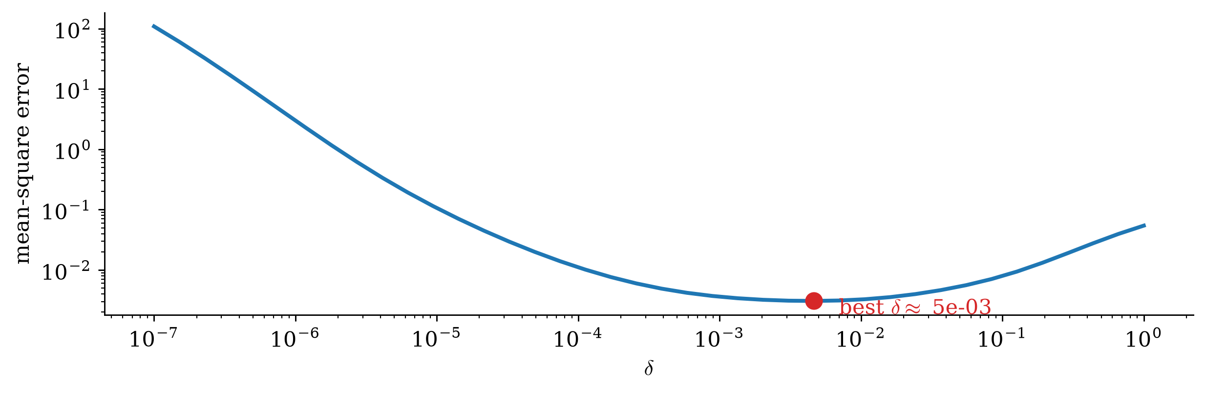
Too little: the noise explodes. Too much: the signal is flattened. The best \(\delta\) is the noise-to-signal ratio of the prior, \(\sigma_N^2/\sigma_X^2\) per component, which the probabilistic reading hands you and the purely deterministic one does not.

Every penalty is a prior

penalty	name	what it assumes about \(\mathbf x\)
\(\norm{\mathbf x}_2^2\)	ridge, Tikhonov	Gaussian: small, spread out
\(\norm{\mathbf x}_1\)	lasso	Laplacian: mostly zero
a mix of the two	elastic net	sparse, but correlated in groups
\(\norm{\mathbf D\mathbf x}_2^2\)	smoothness	small differences between neighbors

A quadratic penalty and a Gaussian prior are the same assumption wearing two hats. The Laplacian prior of the Bayesian week has no closed form, which is why sparse recovery needs its own algorithms.

→ Demo: Gaussian versus Laplacian priors for sparse deconvolution

When is the problem hard? Look at the angles

Spectral unmixing. Left: three known signatures, two nearly alike, and one noisy mixed reading. Middle: the eigenvalues of \(\mathbf A\tran\mathbf A\). Right: concentrations from the naive and the regularized inverse.

Two signatures \(8^\circ\) apart make \(\mathbf A\tran\mathbf A\) nearly singular, and the difference of their concentrations is amplified a hundredfold. Whether an inverse problem is hard can be read off the forward model before any data arrive.

Denoising: the simplest forward model

\(\mathbf A=\mathbf I\): observe the signal itself in white noise, \(\mathbf Y=\mathbf X+\mathbf N\). Then \(\widehat{\mathbf X}=\mathbf C_{\mathbf{XX}}\paren{\mathbf C_{\mathbf{XX}}+\sigma_N^2\mathbf I}^{-1}\mathbf Y\), and in the KLT coordinates of \(\mathbf C_{\mathbf{XX}}\) it applies independent gains \[g_k=\frac{\lambda_k}{\lambda_k+\sigma_N^2}\in(0,1).\]

Figure 9: Left: the denoising gain against each component’s SNR. Right: the noise floor as a lift of every eigenvalue.

Noise regularizes

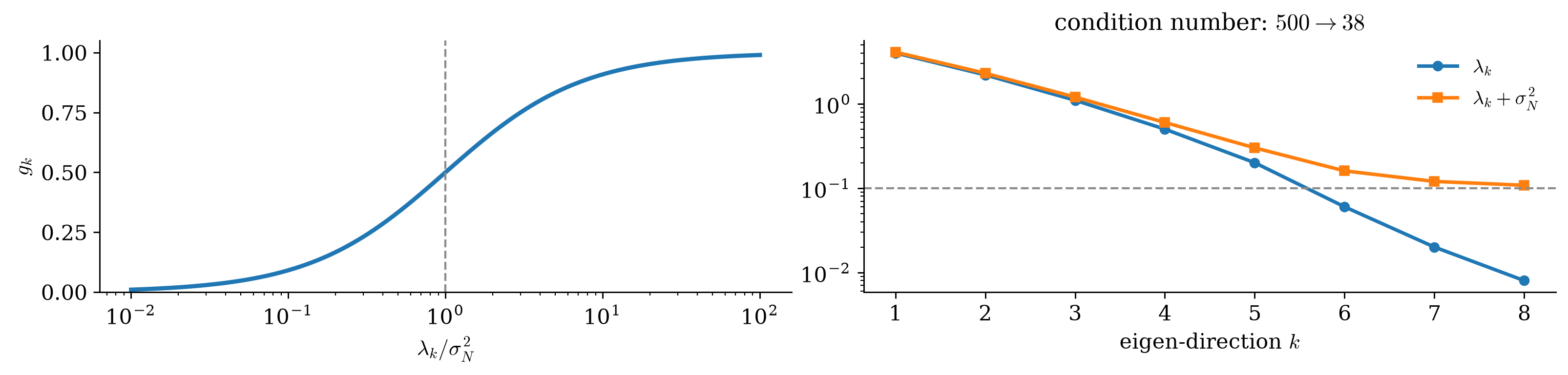
The estimator inverts not \(\mathbf C_{\mathbf{XX}}\) but \(\mathbf C_{\mathbf{XX}}+\sigma_N^2\mathbf I\): every eigenvalue lifted by the noise power. That is ridge, with \(\delta=\sigma_N^2\).

Strong components pass almost untouched, weak ones are shrunk: shrinkage, not thresholding, the scalar shrinkage of the Bayesian week once per eigenvalue.

Regularization is not a trick It is what optimal estimation does on its own once the observation is admitted to be noisy.

Colored noise lifts each direction by its own power; prewhitening restores the uniform case.

Sensor fusion

Several sensors, partial views

Back to the estimation letters: \(\mathbf Y\) the unknown, \(\mathbf X_i\) the readings. \[\mathbf X_i=\mathbf H_i\mathbf Y+\mathbf N_i,\qquad i=1,\dots,M,\] independent noises \(\mathbf R_i\), and a prior \((\mathbf m_0,\mathbf P_0)\).

One sought cause, several known views of it, each with its own noise. A direction no \(\mathbf H_i\) looks along gets certainty from no sensor.

Precisions add

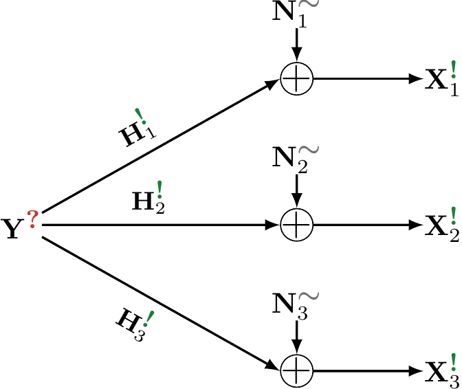
Stack the sensors into one tall inverse problem; the answer is cleanest in information form:

Information form \[\mathbf P^{-1}=\mathbf P_0^{-1}+\sum_i\mathbf H_i\herm\mathbf R_i^{-1}\mathbf H_i ,\qquad \widehat{\mathbf Y}=\mathbf P\paren{\mathbf P_0^{-1}\mathbf m_0+\sum_i\mathbf H_i\herm\mathbf R_i^{-1}\mathbf X_i}.\]

Two thermometers, promoted to matrices: precisions add, the prior is one more measurement, and each sensor is weighted by \(\mathbf R_i^{-1}\) times its signature \(\mathbf H_i\).

The information form is Fisher information

For Gaussian noise the log-likelihood of all sensors together is a sum, and its curvature in \(\mathbf Y\) is \(\mathbf I(\mathbf Y)=\sum_i\mathbf H_i\herm\mathbf R_i^{-1}\mathbf H_i\).

Precision adds information \[\mathbf P^{-1}=\mathbf P_0^{-1}+\mathbf I(\mathbf Y):\] posterior precision is prior precision plus Fisher information. Without a prior the fused covariance is the Cramér–Rao bound, attained.

The floor of the scalar week, for a vector parameter observed by many instruments. Information adds over sensors exactly as it added over samples.

Complementary sensors

Figure 10: Two sensors, each measuring one direction well and the other hardly at all (2σ ellipses), and their fusion.

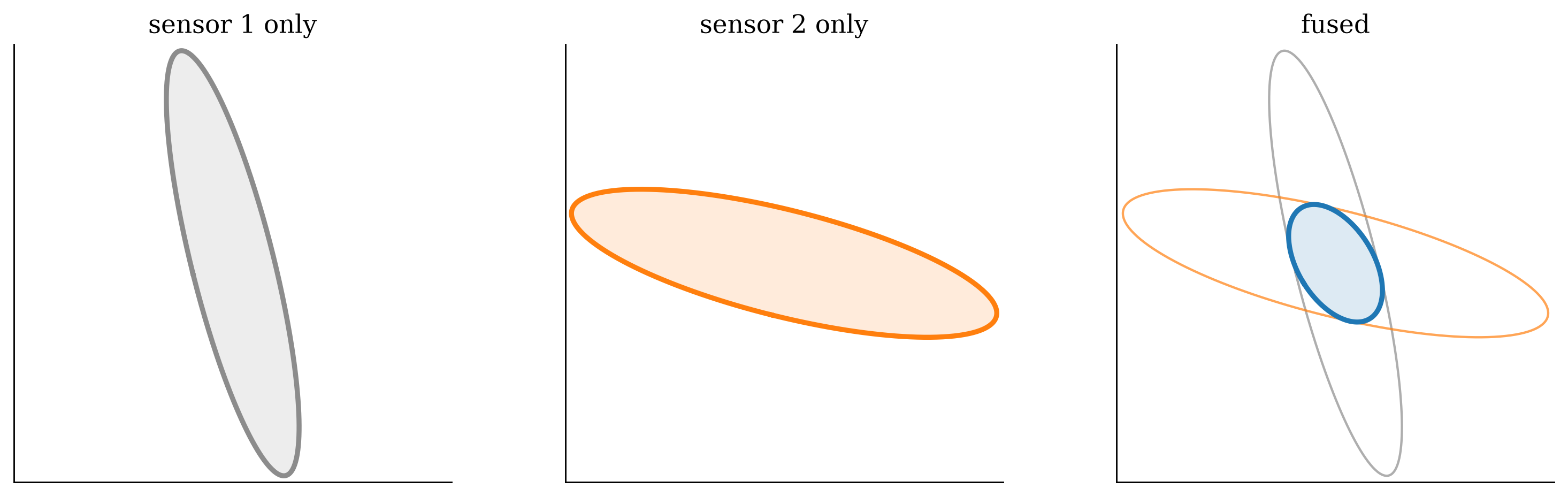
Each \(\mathbf H_i\herm\mathbf R_i^{-1}\mathbf H_i\) is rank one: certainty only along the direction that sensor sees. Neither alone pins the unknown down; together they do.

→ Demo: two directional sensors, precisions that add, and sequential fusion

Diminishing returns

Figure 11: Total error variance trace(P) of a 3-dimensional unknown against the number of fused scalar sensors, each looking along a random direction, for three noise levels.

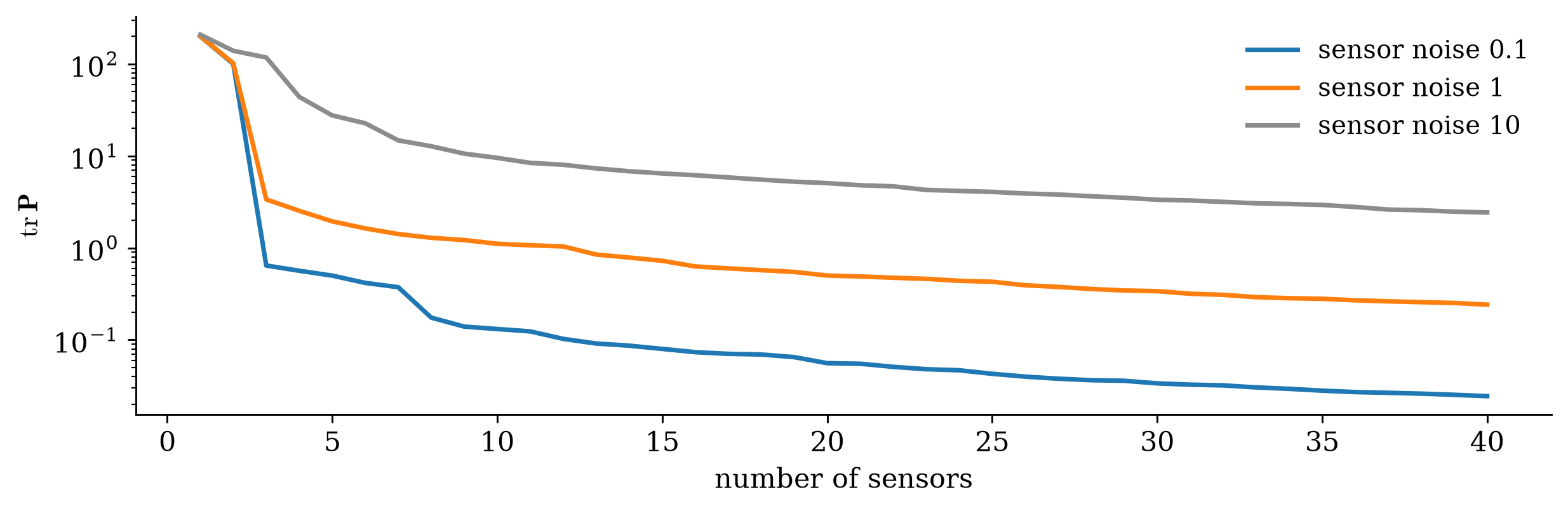
Until three independent directions have been seen, the error is set by the prior. After that each new sensor adds a little less: the error falls like \(1/M\), as for the average of independent readings.

Satellite and inertial navigation

Fusing complementary sensors Unknown: position and velocity, \(\mathbf Y=[P,V]\tran\). A satellite fix measures position only, \(\mathbf H_1=[1\ 0]\); an inertial unit measures velocity only, \(\mathbf H_2=[0\ 1]\). With no prior, \[\mathbf P^{-1}=\begin{bmatrix}\sigma_g^{-2}&0\\0&0\end{bmatrix}+\begin{bmatrix}0&0\\0&\sigma_a^{-2}\end{bmatrix} =\diag\paren{\sigma_g^{-2},\sigma_a^{-2}} .\]

Each summand is singular; the sum is not. Whenever two instruments fail in different directions, the information form says how much each should count, and the answer is never “average them”.

The one formula

instrument	known signature	answer
matched filter	template \(\mathbf u\)	\(\mathbf R_{\mathbf{NN}}^{-1}\mathbf u\)
MVDR beamformer	steering vector \(\mathbf a(\theta_0)\)	\(\mathbf R_{\mathbf{XX}}^{-1}\mathbf a\,/\,\mathbf a\herm\mathbf R_{\mathbf{XX}}^{-1}\mathbf a\)
regularized inverse	forward model \(\mathbf A\)	\(\mathbf P_0\mathbf A\herm(\mathbf A\mathbf P_0\mathbf A\herm+\mathbf R_{\mathbf{NN}})^{-1}\)
fusion	measurement maps \(\mathbf H_i\)	\(\mathbf P\,\mathbf H_i\herm\mathbf R_i^{-1}\)

Whiten with the inverse covariance, then correlate with what you know. Every row is the projection of estimation-as-projection, or its Cauchy–Schwarz twin.

Recap

This week

1. The matched filter whitens, then correlates: \(\mathbf R_{\mathbf{NN}}^{-1}\mathbf u\), the optimal test for Gaussian noise and the best linear score otherwise. In white noise only energy matters; in colored noise, put the signal where the noise is weak.

2. A beamformer is a matched filter for a direction; a bank of them finds sources, and the distortionless constraint turns it into MVDR, which nulls interference it was never told about.

3. An inverse problem needs a prior, and with one the regularized inverse is simply the best linear estimate; noise itself regularizes. Fusion adds precisions. Each instrument is the inverse covariance applied to a known signature.