The Shape of a Random Vector
Covariance is a geometry
Four thousand numbers that move together
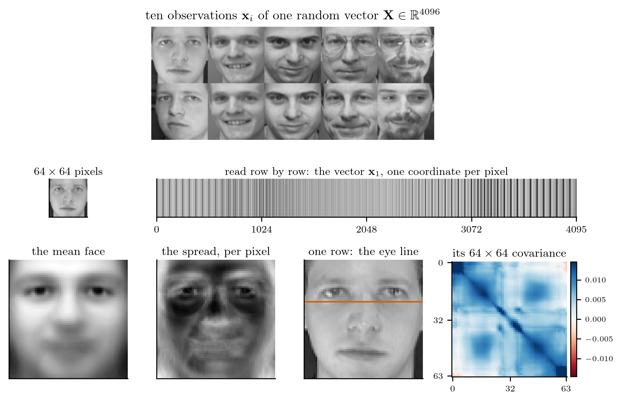
Neighboring pixels are not independent: a face is a shape, and the pixels move together. This week is about describing that shape, and about choosing the coordinates in which it is simplest.
Angle, and Cauchy–Schwarz
\[\abs{\ip{\mathbf x,\mathbf y}}\le\norm{\mathbf x}\,\norm{\mathbf y},\qquad \cos\theta=\frac{\abs{\ip{\mathbf x,\mathbf y}}}{\norm{\mathbf x}\norm{\mathbf y}}\in[0,1] .\]
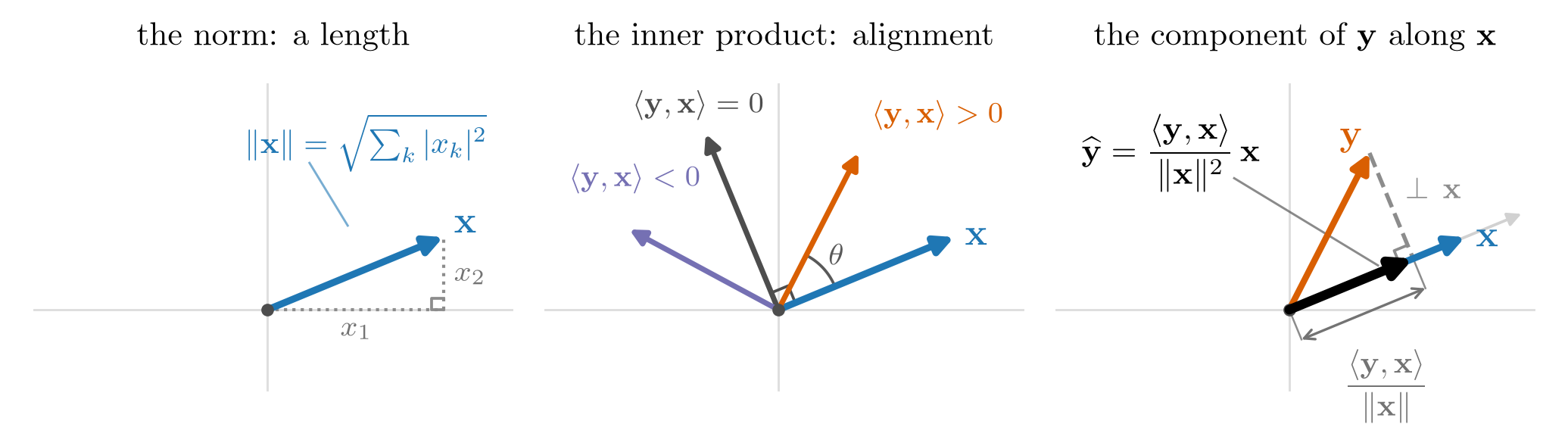
\(\mathbf x\perp\mathbf y\) when \(\ip{\mathbf x,\mathbf y}=0\). That extreme case is the one this course lives on: orthogonality is the algebraic form of “carrying no information about each other”.
Pythagoras and the projection
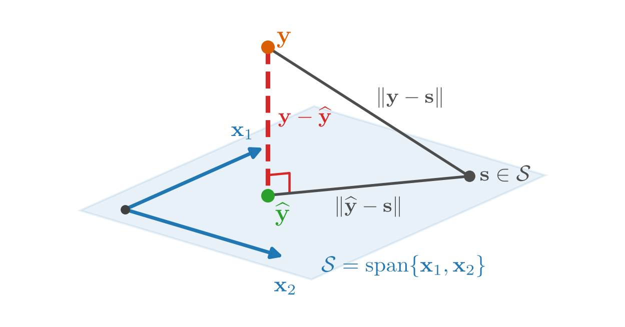
Nothing here used that a vector is a list of numbers, only that there is an inner product. Any space carrying one inherits all of it.
Coordinates in a basis
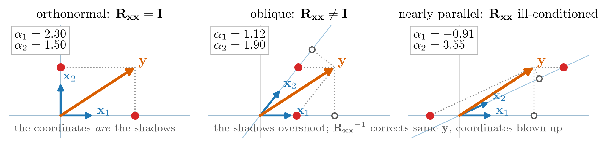
In an orthonormal basis each coefficient is one inner product. In an oblique basis the coefficients come from a linear system whose matrix, the Gram matrix, holds all the pairwise inner products of the basis.
Functions are vectors too
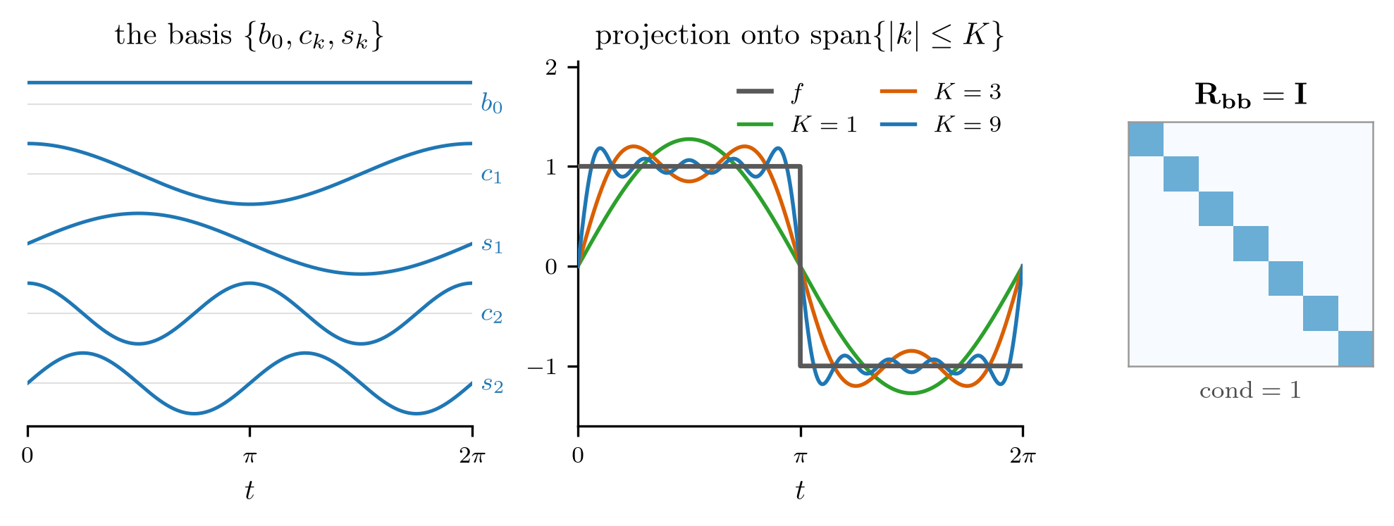
With \(\ip{f,g}=\int f\,g\conj\), a function is a vector with a continuum of coordinates. The Fourier basis is orthonormal, so adding a harmonic never changes the earlier coefficients.
Same subspace, two bases
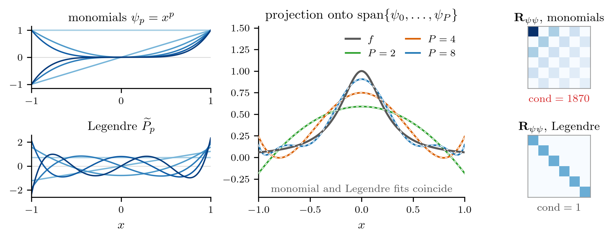
The projection depends only on the subspace; the basis only changes how hard it is to compute. Keep that distinction: this week is about choosing good bases.
A population as three vectors
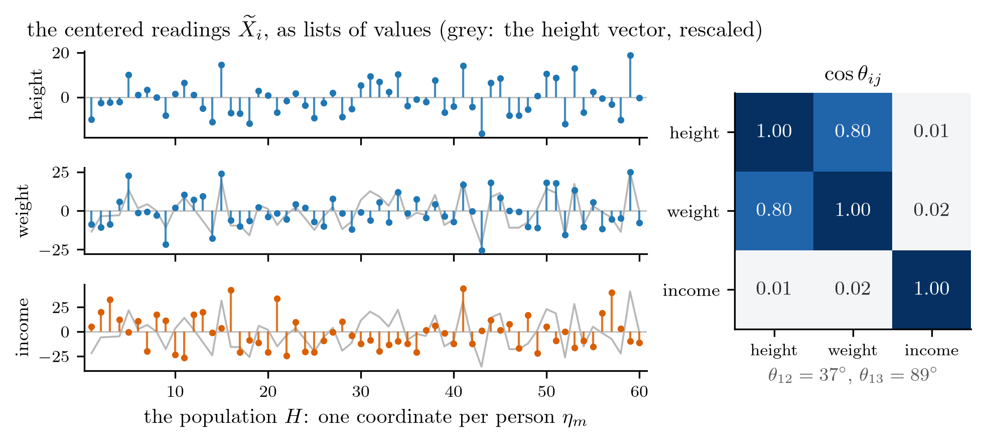
A zero-mean random variable is such a list, with one coordinate per outcome, weighted by its probability. Weight follows height; income does not. That is an angle.
Only the angles enter
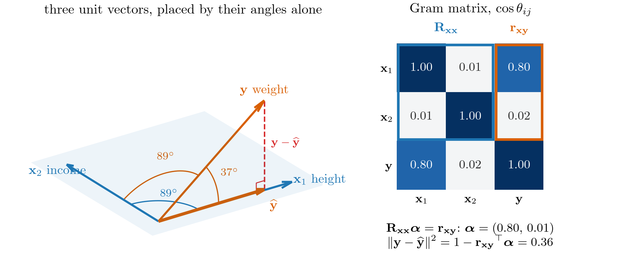
\(\mathbf R_{\mathbf{xx}}\) and \(\mathbf r_{\mathbf{xy}}\) are inner products, not coordinates: the projection depends on the pairwise angles, whatever the dimension of the vectors.
Covariance is variance for a pair
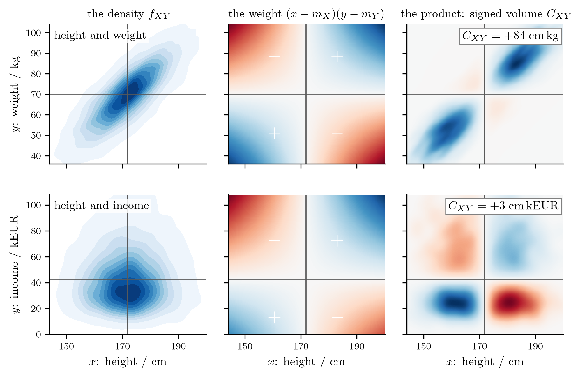
The correlation coefficient is a cosine
Cauchy–Schwarz applied to the centered variables, with \(\ip{U,V}=\E{UV\conj}\): \[\abs{C_{XY}}\le\sigma_X\sigma_Y\quad\Longrightarrow\quad\abs{\rho_{XY}}\le1,\] with equality exactly when \(Y\) is an affine function of \(X\).
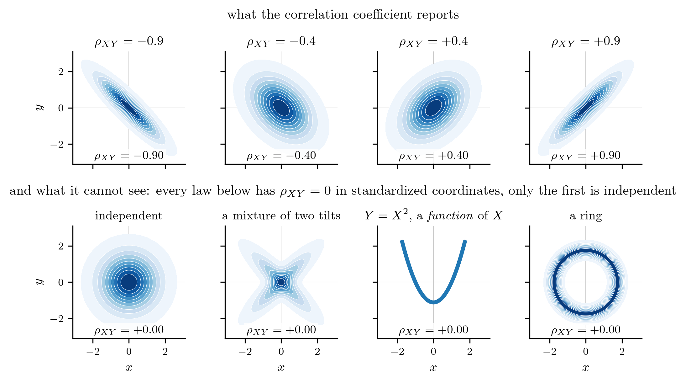
Uncorrelated is not independent
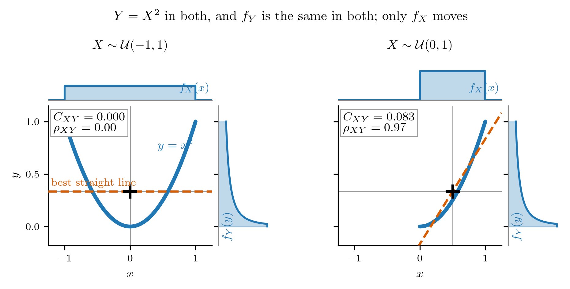
Covariance sees only the straight-line part of the dependence. Zero covariance means “no linear relationship”, not “no relationship”.
Orthogonal is not uncorrelated
\(X,Y\) are uncorrelated when \(C_{XY}=0\), orthogonal when \(R_{XY}=\E{XY\conj}=0\). They differ by the means: \(C_{XY}=R_{XY}-m_Xm_Y\conj\).
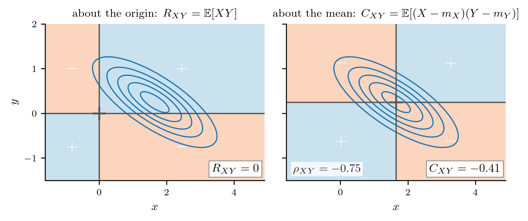
independent \(\Rightarrow\) uncorrelated \(\overset{\text{zero mean}}{\iff}\) orthogonal, and no arrow reverses in general. This is why the course mostly works with zero-mean variables.
How many measurements do you really have?
The variance of a sum keeps its cross terms: \[\Var{\overline X_N}=\frac{1}{N^2}\sum_{k,l}C_{X_kX_l} =\frac{\sigma^2}{N_{\text{eff}}},\qquad N_{\text{eff}}=\frac{N}{1+(N-1)\rho}\] for a common correlation \(\rho\) between any two readings.
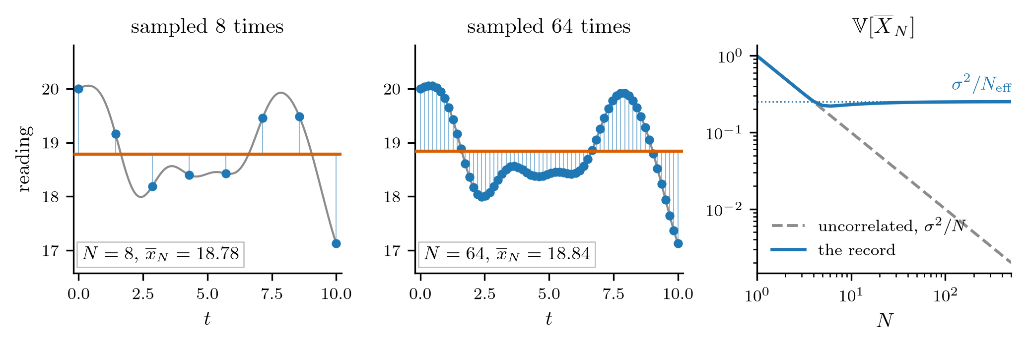
Correlated readings repeat each other. With \(\rho=0.5\), a million readings are worth two. The \(1/\sqrt N\) of independent averaging was a property of independence, not of averaging.
The covariance matrix is a shape
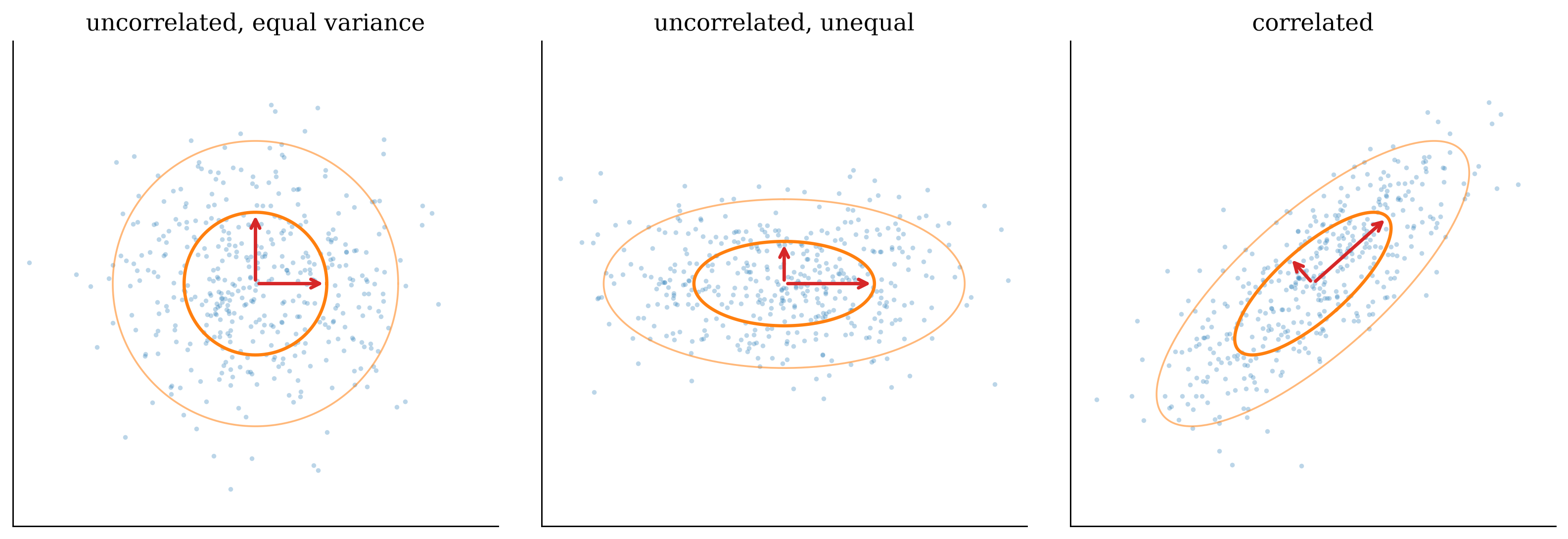
Uncorrelated components: the ellipse is axis-aligned. Correlation tilts it. Decorrelating the data means diagonalizing \(\mathbf C_{\mathbf{XX}}\), an eigenproblem and nothing more.
The variance in every direction
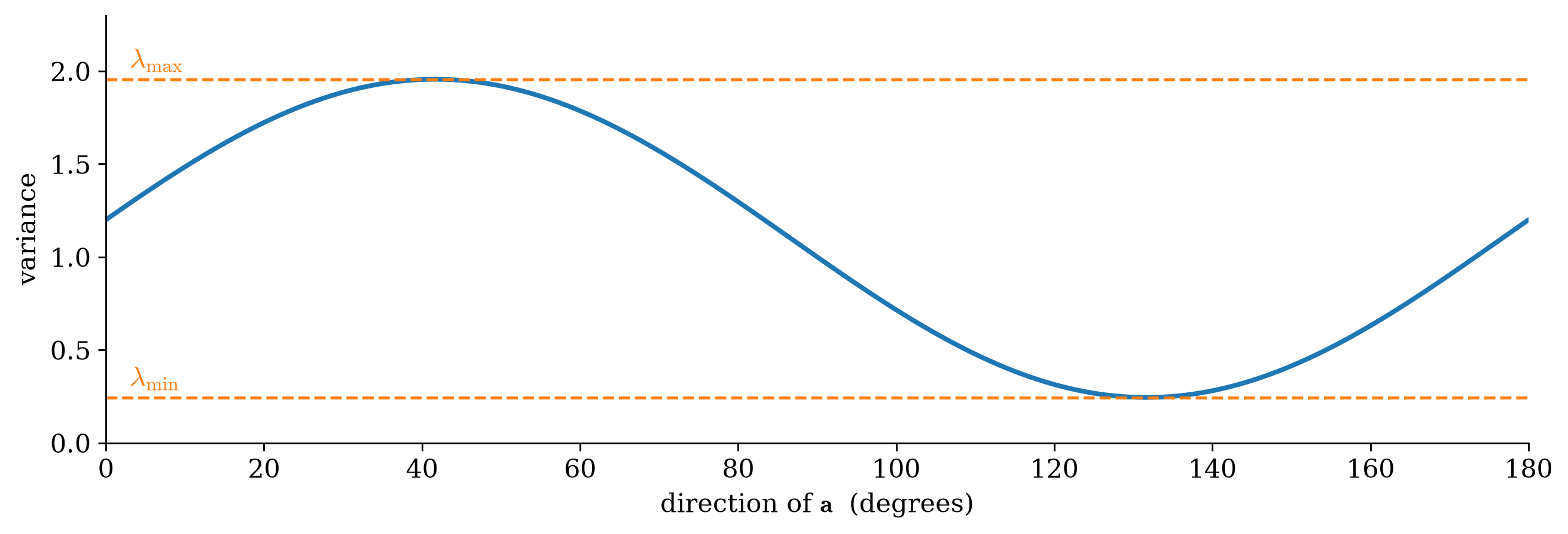
Every direction has its own marginal
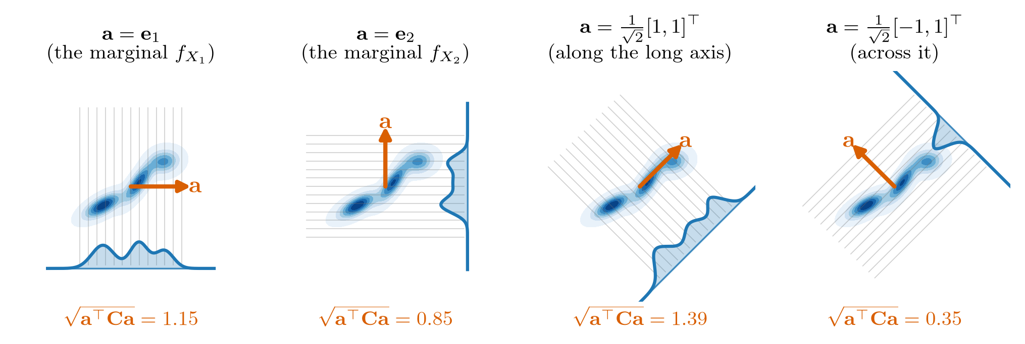
The extremes are the eigenvalues, reached along the eigenvectors; every other direction is trapped between them.
Distance in the data’s own units
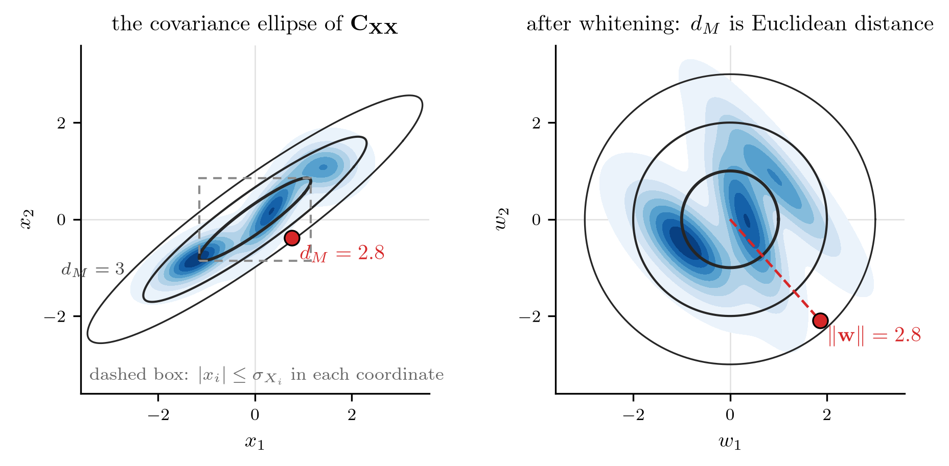
An outlier cannot be judged coordinate by coordinate: this point is unusual because it disobeys the correlation the rest of the data obey.
The covariance matrix from data
\[\widehat{\mathbf m}_{\mathbf X}=\frac1M\sum_m\mathbf x^{(m)},\qquad \widehat{\mathbf C}_{\mathbf{XX}}=\frac{1}{M-1}\sum_m(\mathbf x^{(m)}-\widehat{\mathbf m}_{\mathbf X})(\mathbf x^{(m)}-\widehat{\mathbf m}_{\mathbf X})\herm:\] a sum of rank-one outer products, positive semidefinite by construction.
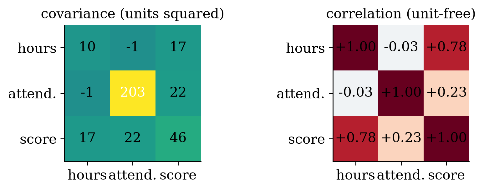
The largest covariance tells you which variable has the biggest units, not which relationship is strongest. Normalizing to correlations makes the matrix readable.
Complex random variables: the conjugate matters
\(Z=X+jY=Re^{j\Phi}\) is a pair of real variables on one outcome, and its size is measured with a conjugate: \(\E{ZZ\conj}=\E{\abs Z^2}\ge0\).
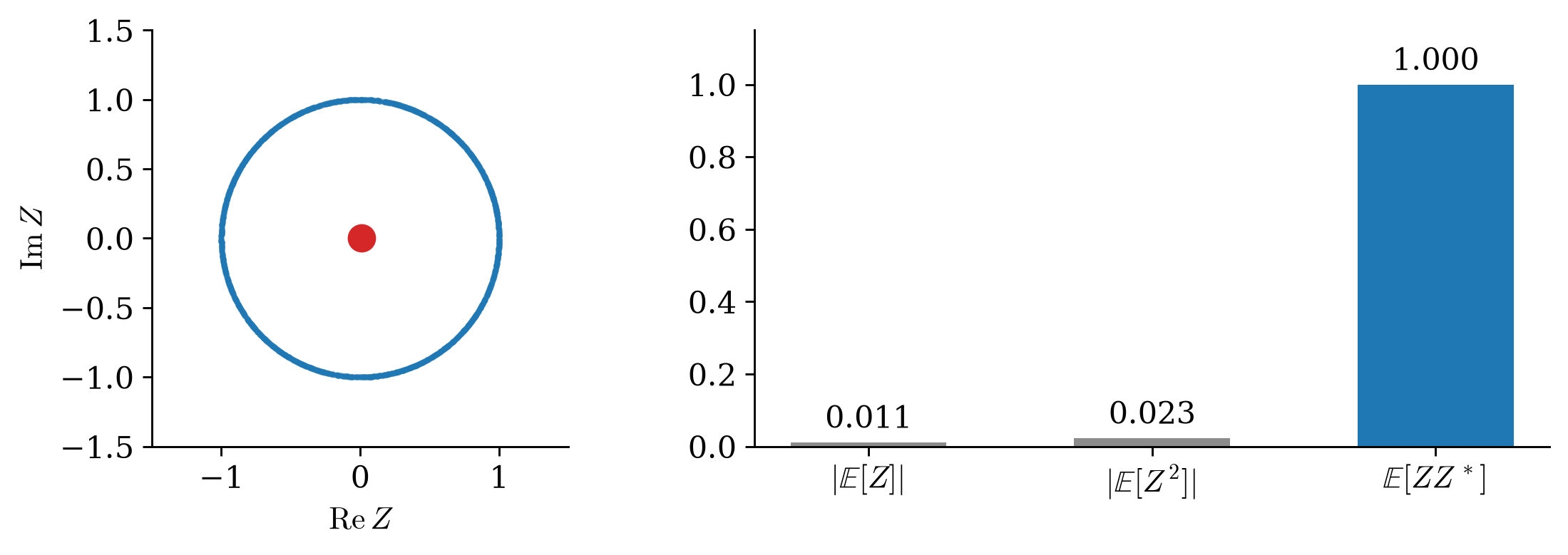
Without the conjugate, the second moment of a phase-rotating signal vanishes however large the signal is. With it, \(\mathbf C_{\mathbf{ZZ}}=\E{(\mathbf Z-\mathbf m)(\mathbf Z-\mathbf m)\herm}\) is Hermitian and positive semidefinite, exactly as in the real case.
Proper: one matrix is enough
\(\mathbf Z=\mathbf X+j\mathbf Y\) has \(2N\) real degrees of freedom; the missing half is the complementary covariance \(\widetilde{\mathbf C}_{\mathbf{ZZ}}=\E{(\mathbf Z-\mathbf m)(\mathbf Z-\mathbf m)\tran}\). A vector is proper when it vanishes.
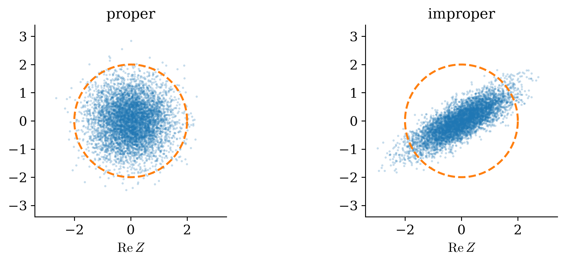
Properness is rotational symmetry: no phase is privileged. A uniformly random carrier phase produces it, which makes it the standard model for communication and array signals.
Where proper signals come from
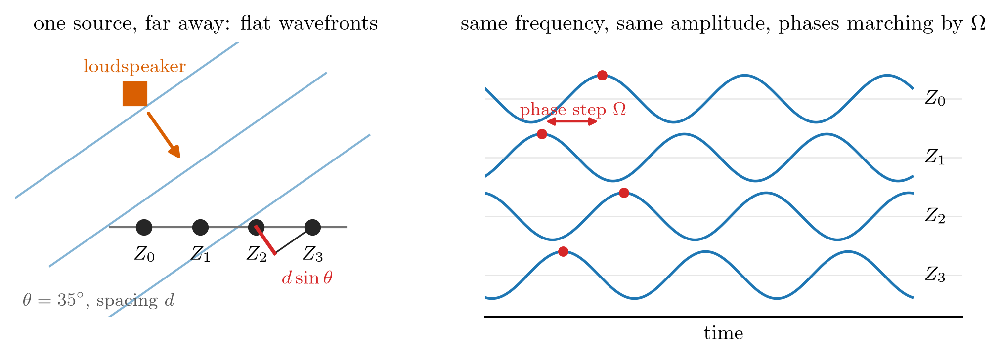
The snapshot is \(\mathbf Z=Ae^{j\Theta}\mathbf v+\mathbf N\) with \(\Theta\) uniform. Its covariance \(\abs A^2\mathbf v\mathbf v\herm+\sigma_N^2\mathbf I\) is one strong direction lifted above an isotropic noise floor.
The unknown absolute phase is what makes the snapshot proper, and the rank-one term is where the direction of the source is written.
Three elementary maps
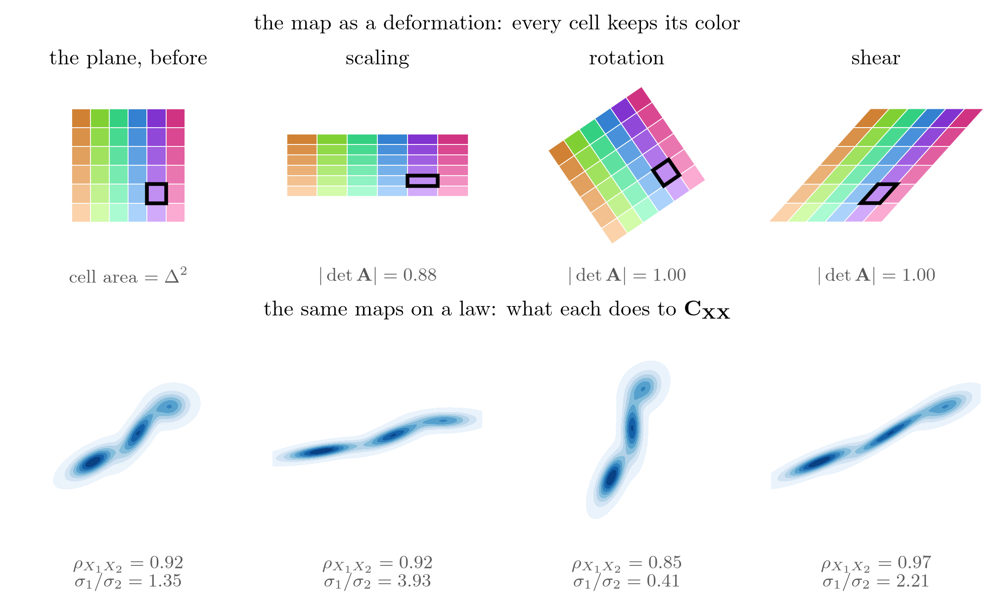
Scaling changes variances and leaves the correlation coefficient alone. A rotation keeps every length and eigenvalue and changes only which direction is which. A shear creates correlation.
Choosing \(\mathbf A\) is the whole game
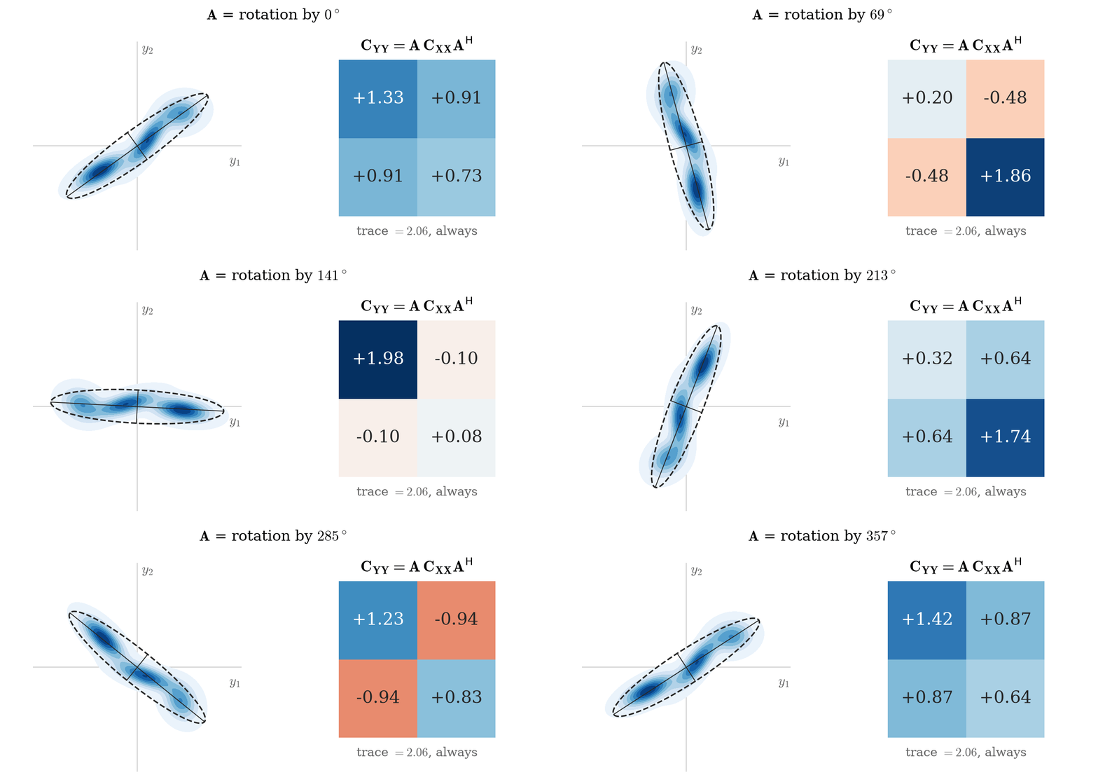
In \(\mathbf C_{\mathbf{YY}}=\mathbf A\mathbf C_{\mathbf{XX}}\mathbf A\herm\), choose \(\mathbf A\) to make
- \(\mathbf C_{\mathbf{YY}}\) diagonal: the outputs are uncorrelated (decorrelation);
- \(\mathbf C_{\mathbf{YY}}=\mathbf I\): uncorrelated and of unit scale (whitening);
- \(\mathbf C_{\mathbf{YY}}\) equal to a target: a signal with prescribed statistics (coloring).
The natural axes: eigenvectors
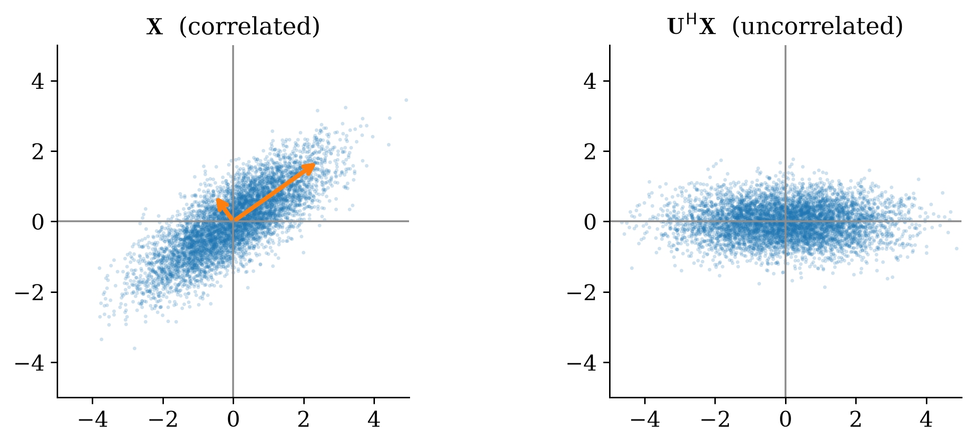
\[\mathbf C_{\mathbf{XX}}=\mathbf U\boldsymbol\Lambda\mathbf U\herm,\qquad \mathbf U\herm\mathbf U=\mathbf I,\quad \lambda_i\ge0 .\]
Hermitian gives the orthonormal \(\mathbf U\); positive semidefinite gives \(\lambda_i\ge0\). Transform by \(\mathbf U\herm\): \(\mathbf C_{\mathbf{WW}}=\mathbf U\herm\mathbf C_{\mathbf{XX}}\mathbf U=\boldsymbol\Lambda\), diagonal.
Whitening: ellipsoid into sphere
\(\mathbf A\) whitens \(\mathbf X\) if \(\mathbf A\mathbf C_{\mathbf{XX}}\mathbf A\herm=\mathbf I\). The eigenvectors solve it on sight: \(\mathbf A_{\text{PCA}}=\boldsymbol\Lambda^{-1/2}\mathbf U\herm\), rotate, then divide each axis by its own standard deviation.
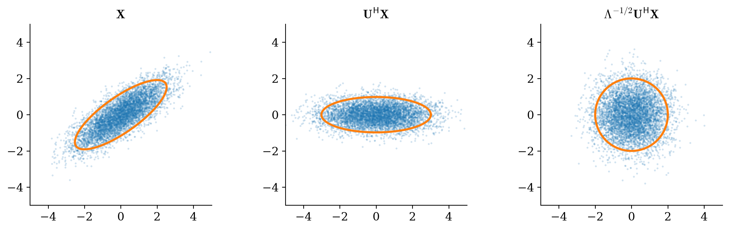
In whitened coordinates the Mahalanobis distance is ordinary Euclidean distance. Whitening is a change of metric, and every \(\mathbf C^{-1}\) that appears later in the course is this change of metric at work.
Three whiteners, three extra properties
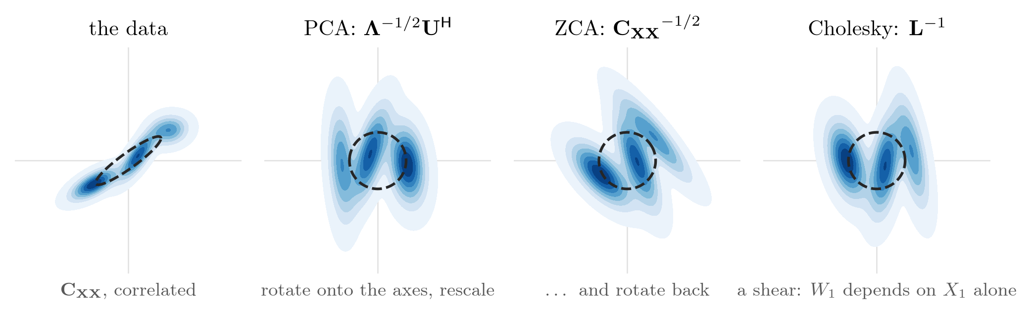
| whitener | \(\mathbf A\) | what else it buys |
|---|---|---|
| PCA | \(\boldsymbol\Lambda^{-1/2}\mathbf U\herm\) | coordinates ordered by variance |
| ZCA | \(\mathbf U\boldsymbol\Lambda^{-1/2}\mathbf U\herm=\mathbf C^{-1/2}\) | the output changes least from the input |
| Cholesky | \(\mathbf D^{-1/2}\mathbf L^{-1}\) | causal: output \(i\) uses only inputs \(1,\dots,i\) |
→ Demo: the covariance ellipse, Mahalanobis distance, and three whiteners
Coloring, drawn
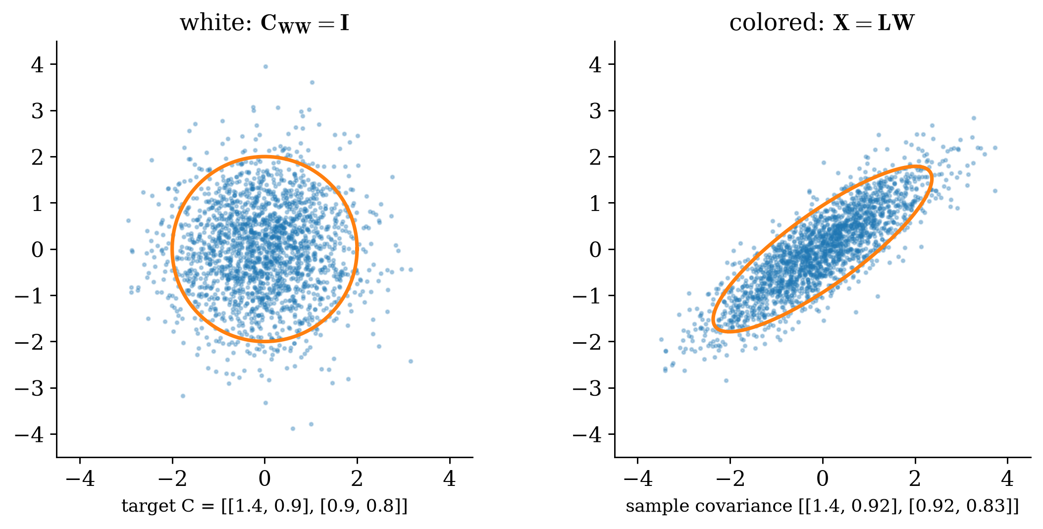
The circle is stretched and sheared into the target ellipse; the sample covariance matches the target. This is how correlated test noise is made.
The spectrum is the price list
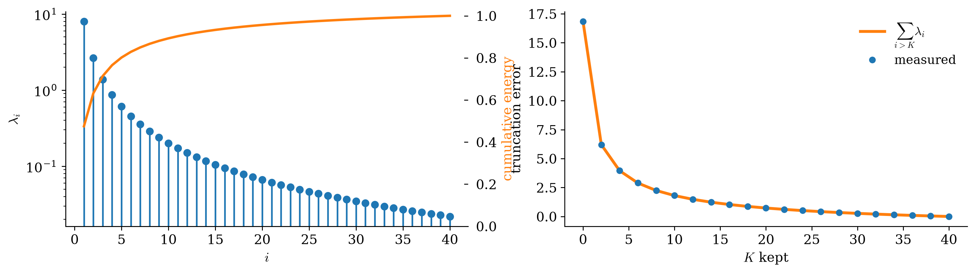
The optimal subspace is unique; the basis inside it is not. Energy compaction fixes the subspace; decorrelation is what singles out the eigenbasis within it.
Eigenfaces
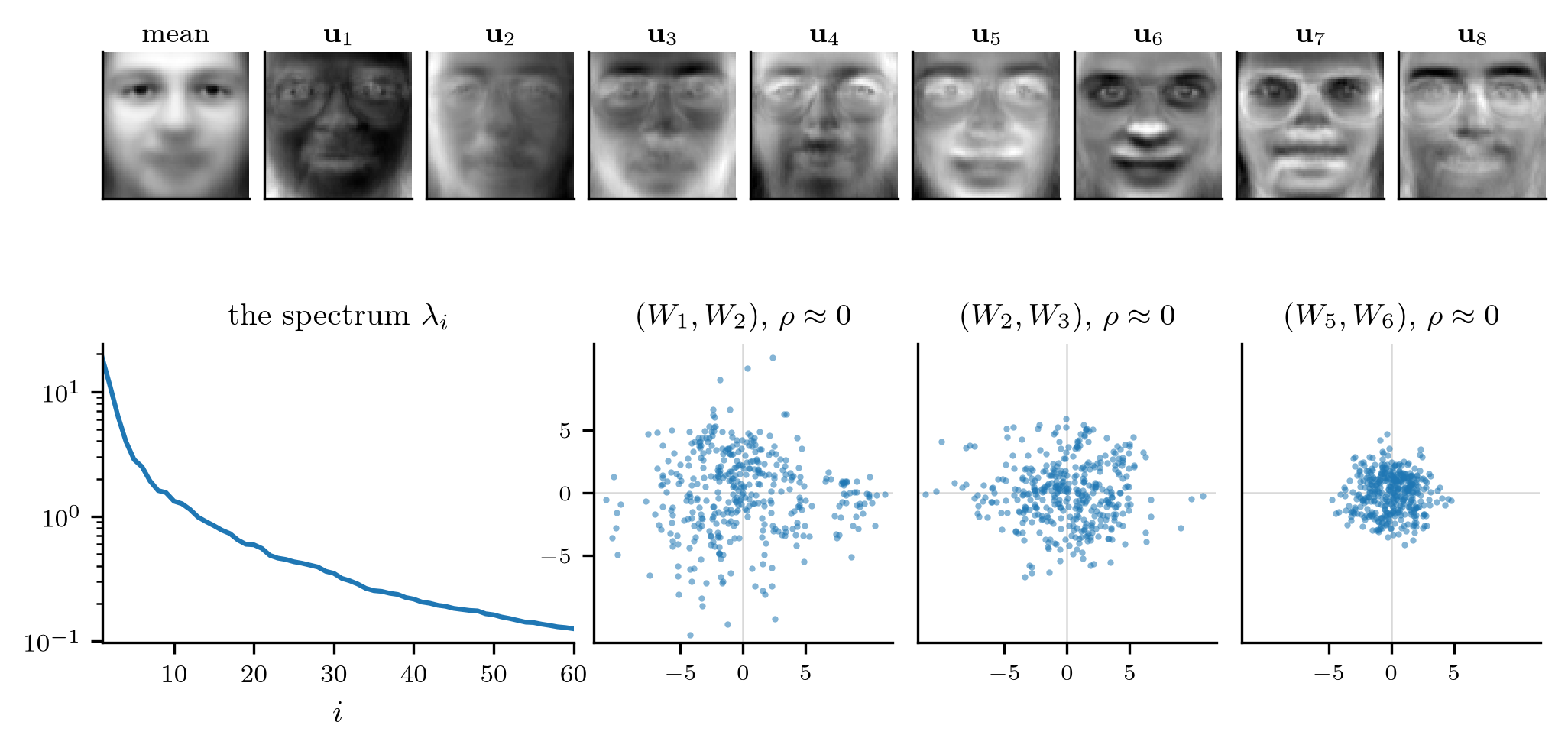
Coarse illumination first, fine detail last. A few dozen numbers describe a face of 4096 pixels, because the pixels move together. Nothing about faces was built into the method: the basis was read off the covariance alone.
Two moments are the whole law
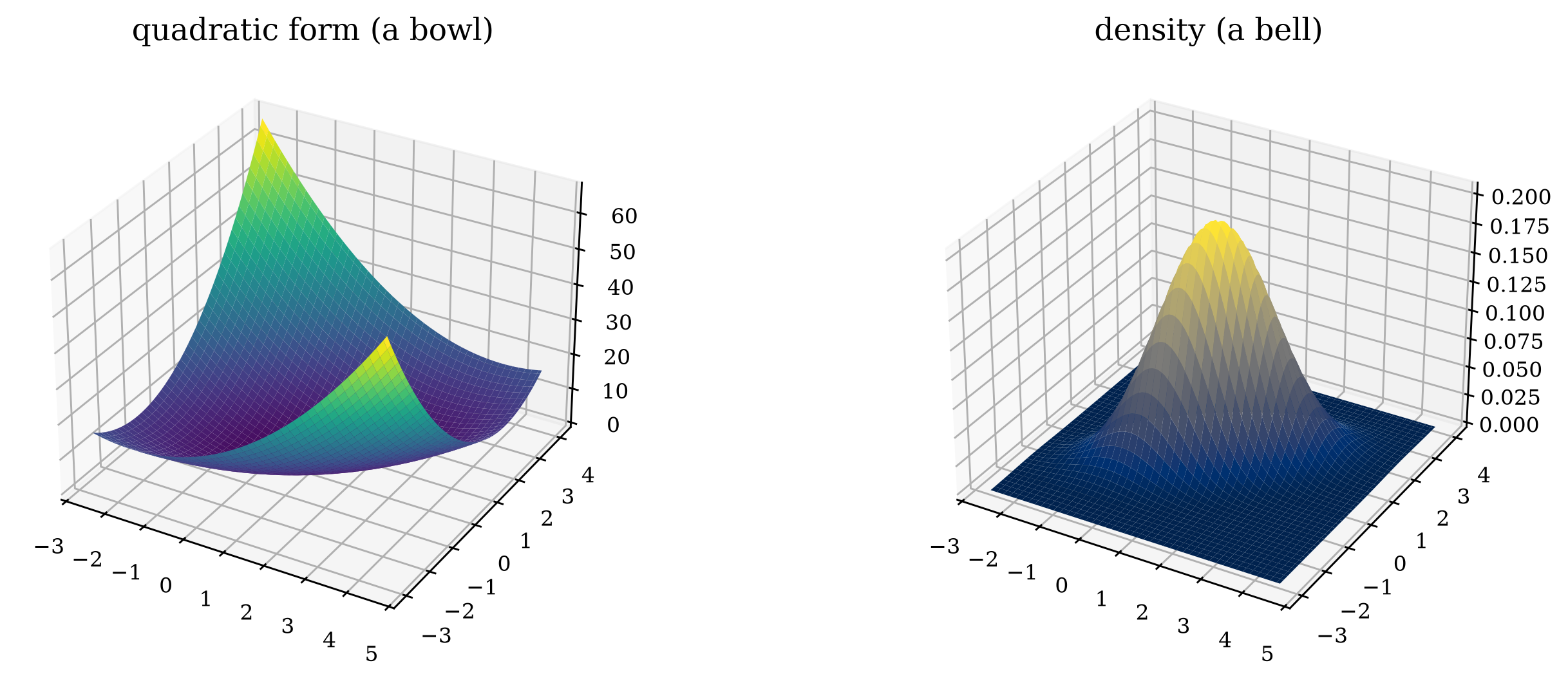
The level sets of the density are exactly the covariance ellipsoids. For a Gaussian vector the mean and the covariance are not a summary; they are everything.
The 68–95–99.7 rule does not survive dimension
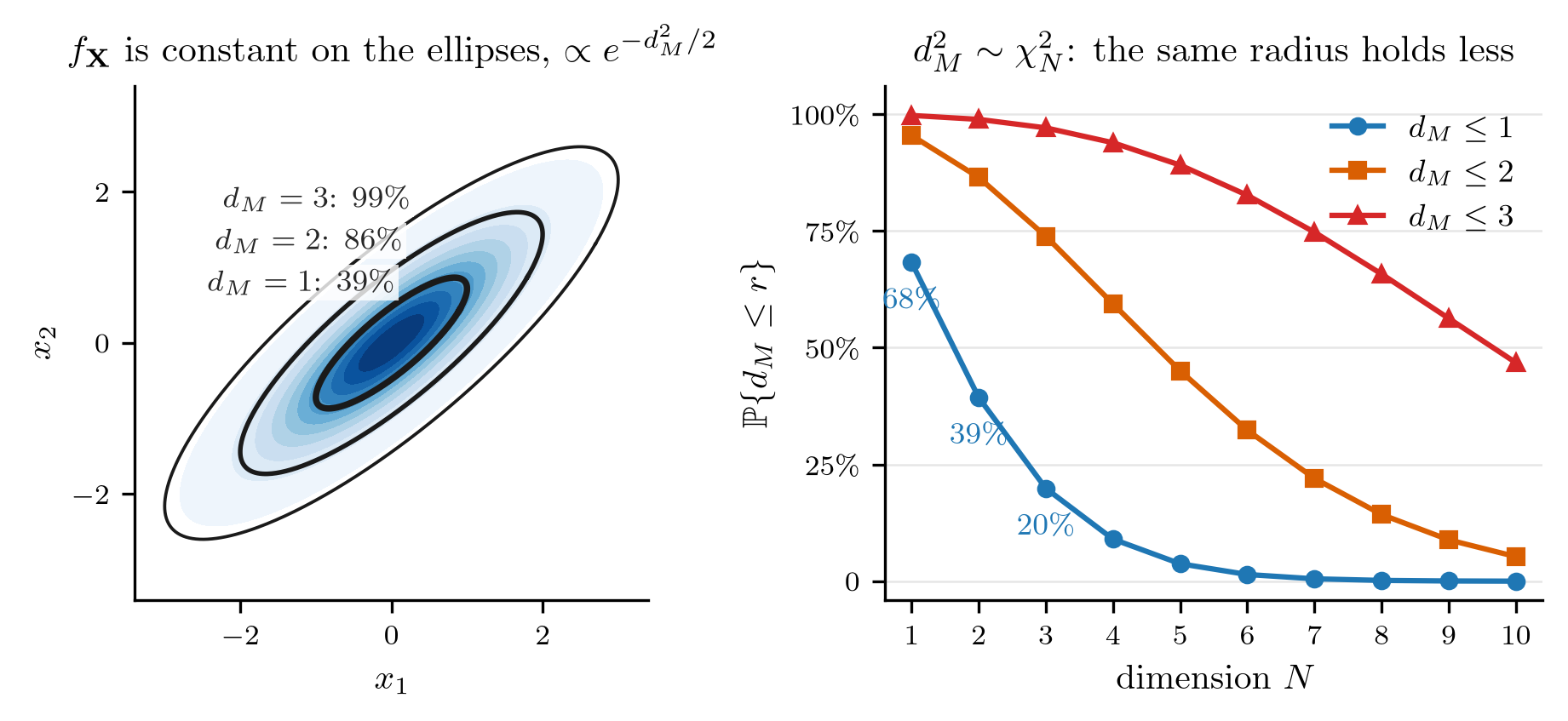
In one dimension \(d_M\le1\) holds 68% of the mass, in two 39%, in three 20%. In high dimension almost all the mass lies far from the mean, measured in standard deviations: estimation gets harder with dimension.
“Jointly” matters
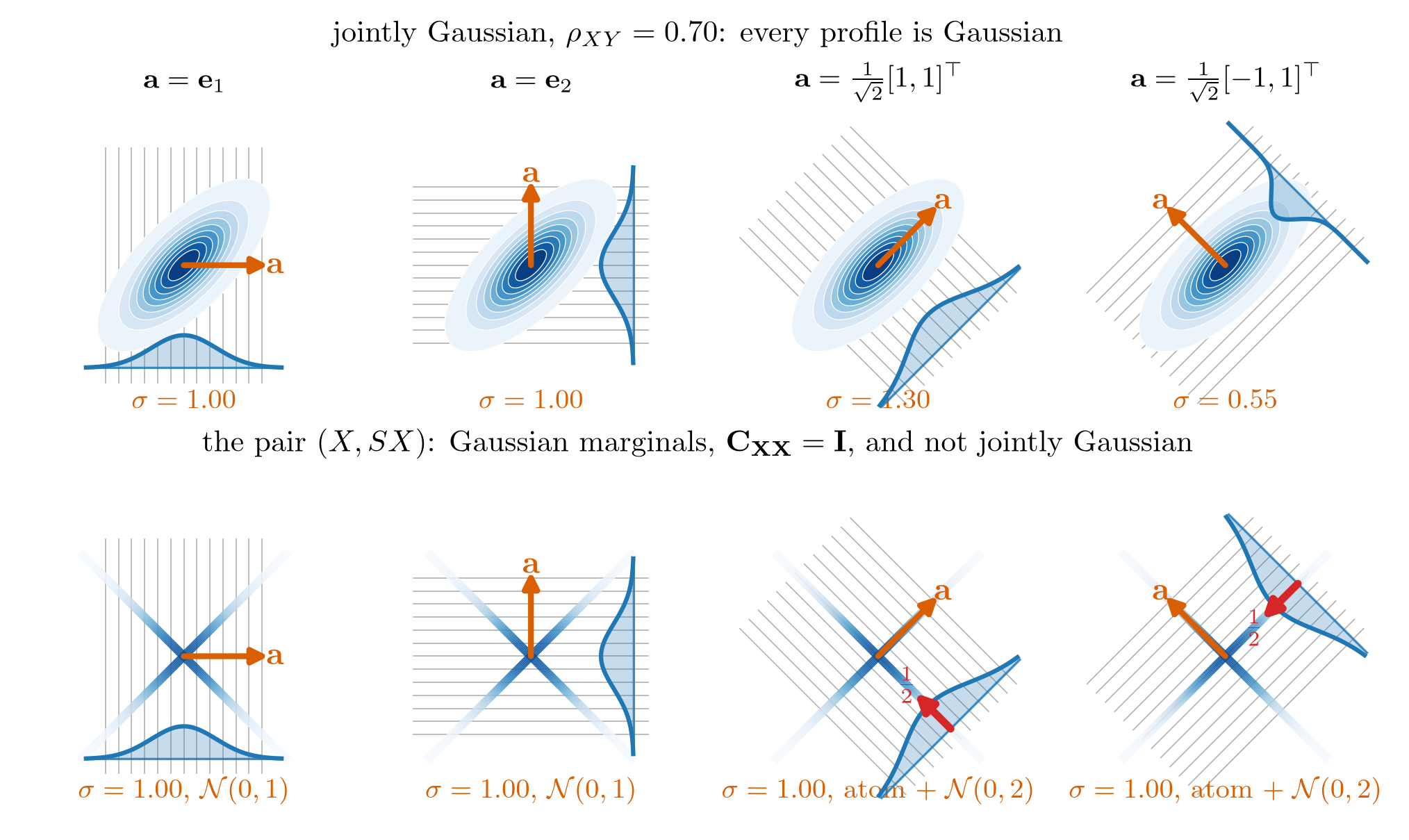
\(\mathbf X\) is jointly Gaussian if and only if every projection \(\mathbf a\herm\mathbf X\) is Gaussian. Two marginals are just two projections out of infinitely many; the diagonal one gives \((X,SX)\) away, since \(X+SX\) is exactly zero half the time.
The proper complex Gaussian
\[f_{\mathbf Z}(\mathbf z)=\frac{1}{\pi^N\det\mathbf C_{\mathbf{ZZ}}} \exp\paren{-(\mathbf z-\mathbf m)\herm\mathbf C_{\mathbf{ZZ}}^{-1}(\mathbf z-\mathbf m)}\]
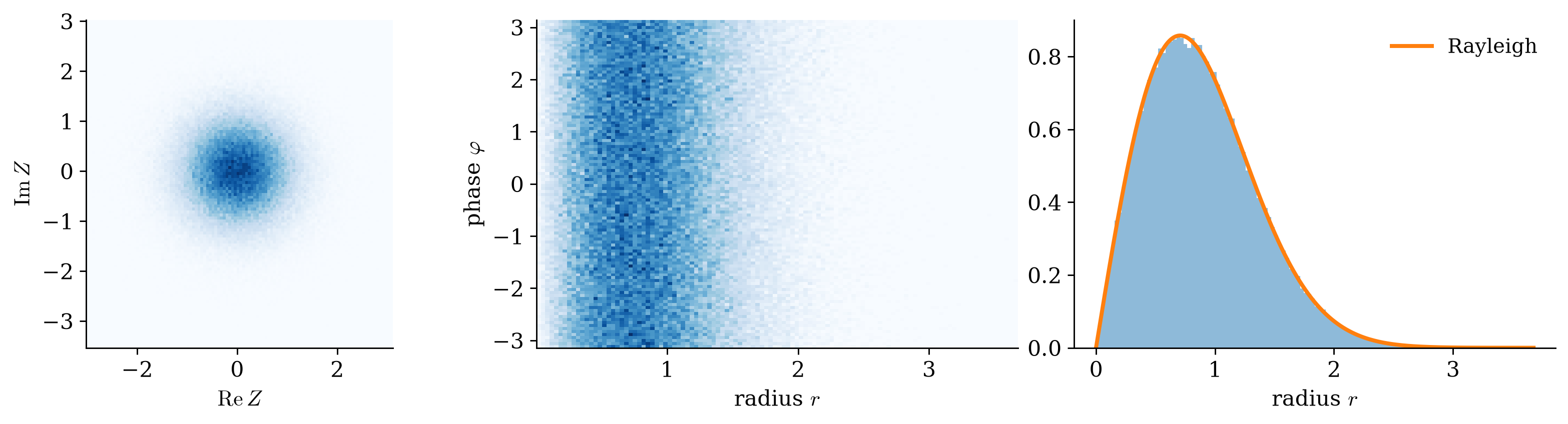
The flat phase panel is properness seen directly. This is the standard model for receiver noise.
Why the model keeps being right
For iid random vectors with finite covariance, the normalized sum is Gaussian: \(\frac{1}{\sqrt n}\sum_i(\mathbf X_i-\mathbf m)\to\Gauss(\mathbf 0,\mathbf C)\). Proof: apply the scalar central limit theorem to every projection \(\mathbf a\herm\mathbf X\).
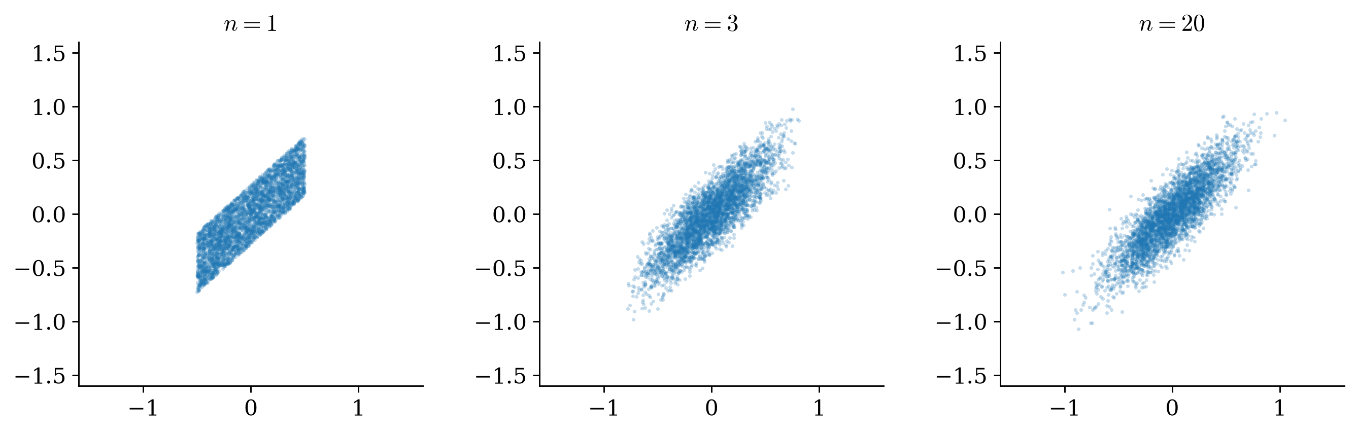
The square becomes an ellipse whose contours are set by \(\mathbf C\) alone: the first week’s answer, now for vectors.