What This Course Is For

Week 0 · A tour of the course

Signals you cannot see directly

\[ % Number sets \newcommand{\Nat}{\mathbb{N}} \newcommand{\Integer}{\mathbb{Z}} \newcommand{\Real}{\mathbb{R}} \newcommand{\Complex}{\mathbb{C}} % Operators \newcommand{\SNR}{\operatorname{SNR}} \newcommand{\tr}{\operatorname{tr}} \newcommand{\re}{\operatorname{Re}} \newcommand{\im}{\operatorname{Im}} \newcommand{\sign}{\operatorname{sign}} \newcommand{\rect}{\operatorname{rect}} \newcommand{\sinc}{\operatorname{si}} \newcommand{\erf}{\operatorname{erf}} \newcommand{\erfc}{\operatorname{erfc}} \newcommand{\kurt}{\operatorname{kurt}} \newcommand{\diag}{\operatorname{diag}} \newcommand{\MSE}{\operatorname{MSE}} \newcommand{\argmin}{\operatorname*{argmin}} \newcommand{\argmax}{\operatorname*{argmax}} \newcommand{\bias}{\operatorname{bias}} \newcommand{\Bin}{\operatorname{Bin}} % Delimiters \newcommand{\paren}[1]{\left(#1\right)} \newcommand{\bracket}[1]{\left[#1\right]} \newcommand{\set}[1]{\left\{#1\right\}} \newcommand{\abs}[1]{\left\lvert #1 \right\rvert} \newcommand{\norm}[1]{\left\lVert #1 \right\rVert} \newcommand{\ip}[1]{\left\langle #1 \right\rangle} % Notation \newcommand{\dd}{\,\mathrm{d}} \newcommand{\tran}{^{\top}} \newcommand{\conv}{\ast} \newcommand{\conj}{^{*}} \newcommand{\herm}{^{\mathsf{H}}} \newcommand{\opt}{^{\star}} % Expectation and variance % \newcommand{\E}[1]{\mathbb{E}\!\left[#1\right]} \newcommand{\E}[2][]{\mathbb{E}_{#1}\!\left[#2\right]} \newcommand{\Var}[1]{\mathbb{V}\!\left[#1\right]} % Distributions \newcommand{\Gauss}{\mathcal{N}} \newcommand{\Uniform}{\mathcal{U}} \newcommand{\FT}{\mathcal{F}} % Probability \newcommand{\Prob}[1]{\mathbb{P}\!\left(#1\right)} % Misc \newcommand{\bsy}[1]{\boldsymbol{#1}} \newcommand{\calR}{\mathcal{R}} \newcommand{\calC}{\mathcal{C}} \]

Corgi or bread?

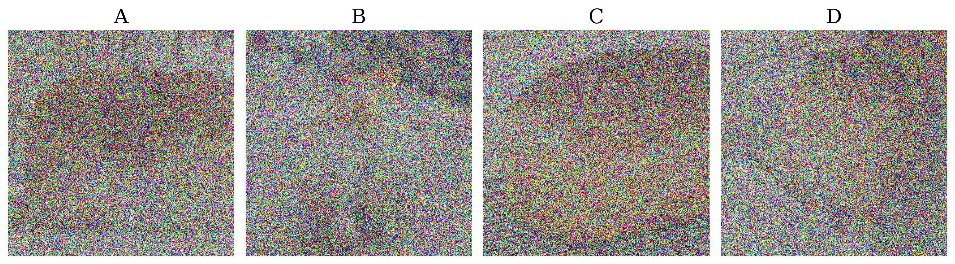
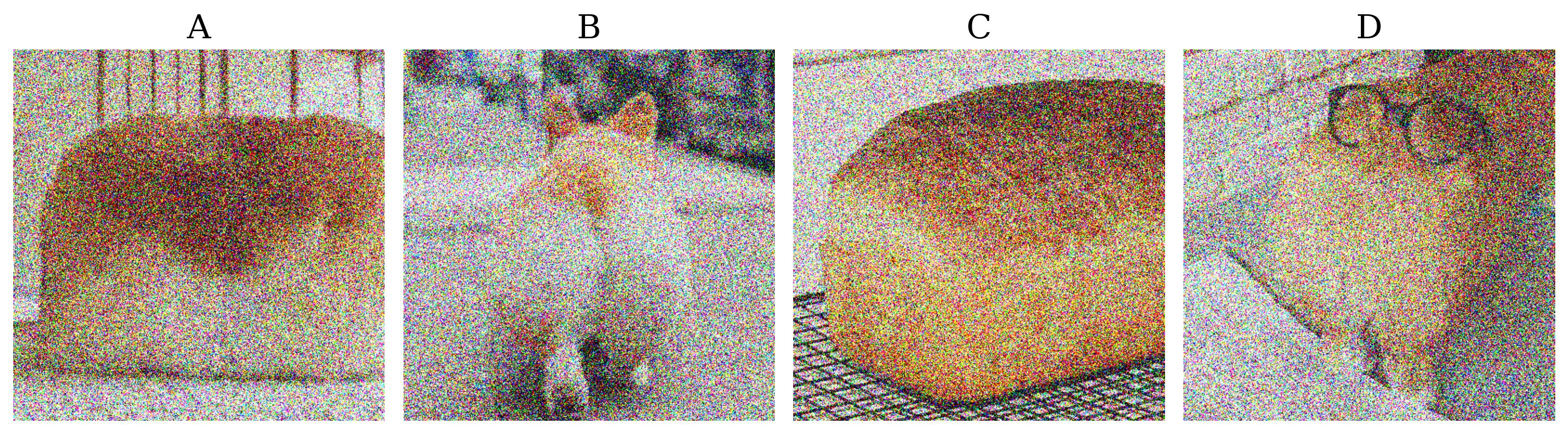
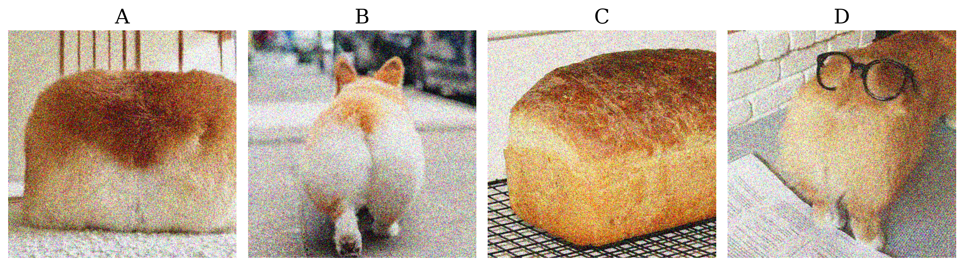
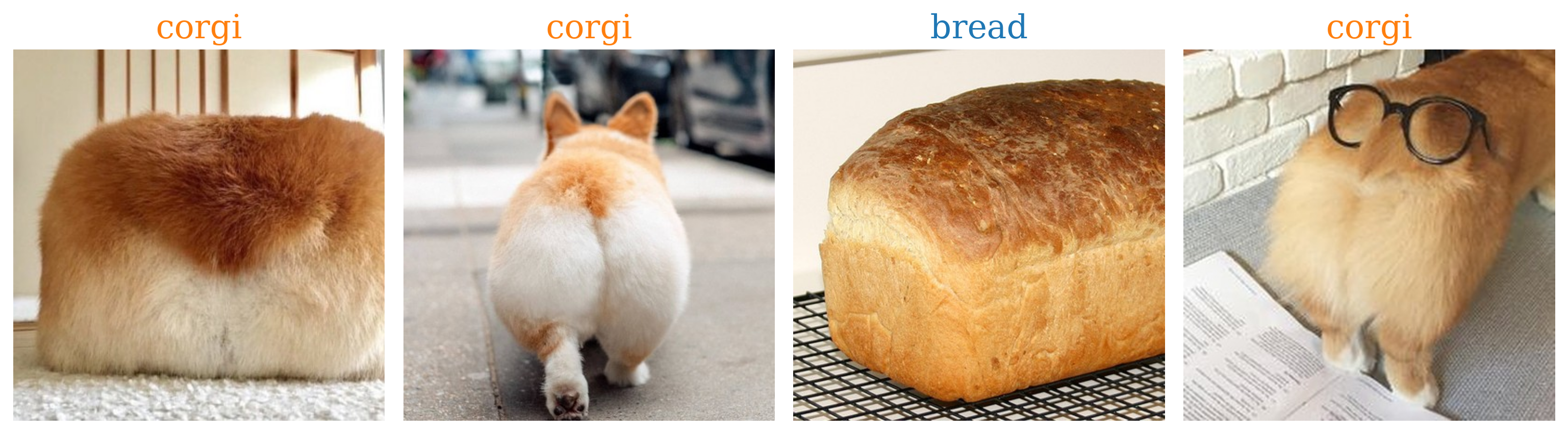
For each photo: corgi or bread, and how sure are you? Say a number between 0 and 100 %.

At each step, a show of hands per photo: who says corgi, who says bread, who would not bet either way. Write the room’s rough percentages on the board and keep them for the next slide. A is a corgi sitting like a loaf; B and D are corgis; C is an honest loaf. Photos from the corgi-or-bread classifier repository (github.com/Kawaeee/butt_or_bread).

What you just did

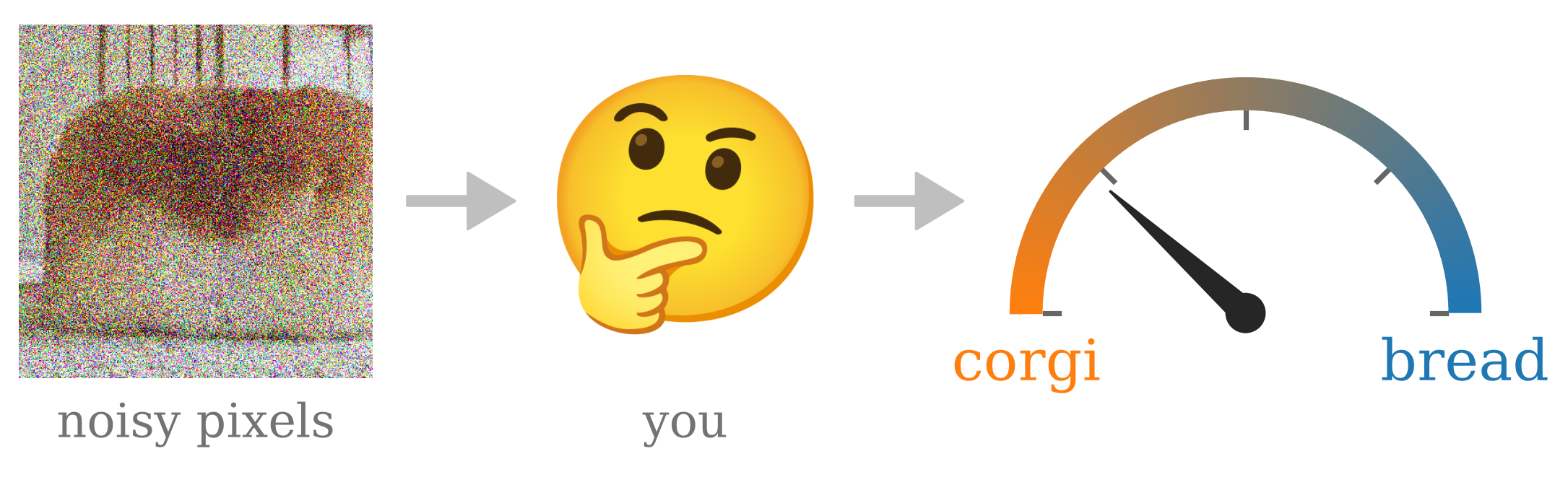
• You never saw a corgi or a loaf, only noisy pixels. Still, you answered, with a confidence.
• You combined what you expected (fur, crust, legs) with what you saw.
• Your confidence moved as the noise went down.

The question of this course How can we know something that we never observe directly? Write down what you expect, what the data say, how to combine them, and how sure you are allowed to be.

Do not name Bayes, likelihood or prior here; when the posterior arrives in week 3, point back to this slide: that is what you did with the corgis.

Your phone did this today

Before you reached this room, it had already:

• found your position from satellite signals about a hundred times weaker than the noise they arrive in,
• kept your own voice from echoing back at you on a call,
• picked your voice out of a noisy kitchen with two or three microphones,
• turned a dark, grainy photo into a clean one.

Estimation None of these measures what it wants. Each computes an estimate from data that is mostly something else: how is it made, and how good can it possibly be?

Ask the room which of the four they think is hardest. The GPS signal arrives about 20 dB below the thermal noise of the receiver; it is recovered by correlating against a known code, the matched filter of week 6. The echo canceller is week 9, the microphone array week 6, the denoiser week 8.

Every measurement is a guess

The short-time spectrum of speech, and the waveform beneath it.

 

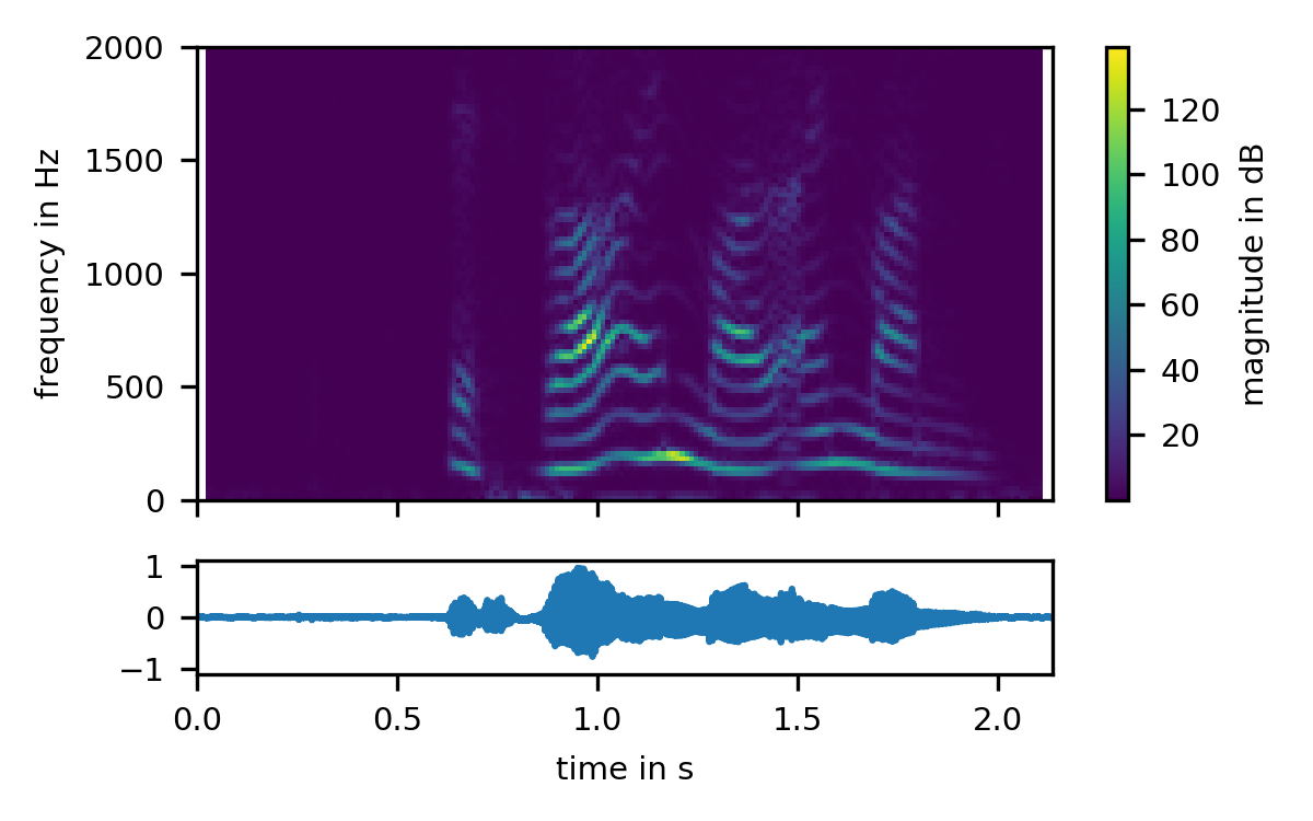
A GPS fix, a microphone signal, an MRI slice, a radar echo: each is the thing we want plus something we do not.

We never get the truth, so we ask for the estimate that is wrong by as little as possible, on average. This course makes that precise, and then solves for it.

What you will be able to do

Compress a face into a few numbers

Figure 1: Top: the mean face and the eight leading eigenfaces, each with the weight this face gives it. Bottom: the running sum. Right: the face, and the sum with 60 terms out of 4096.

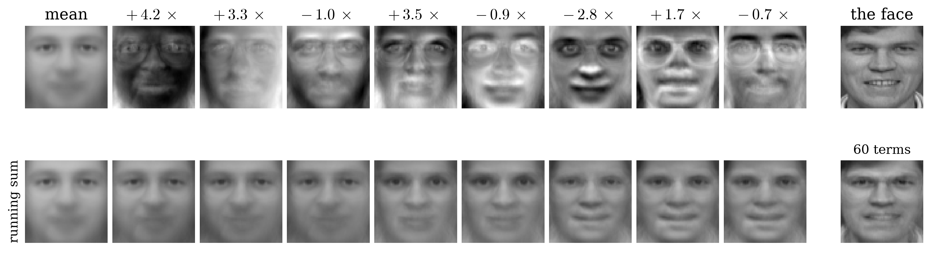
Every face is the mean plus a weighted sum of a few eigenfaces, the directions of the data’s covariance matrix. Eight numbers already say whose face it is. (Week 4)

Fill in the half you did not see

Three portraits the estimator never saw. Left to right: the observed left half, the estimate written into the right half, the truth, the error, and the error predicted in advance.

 

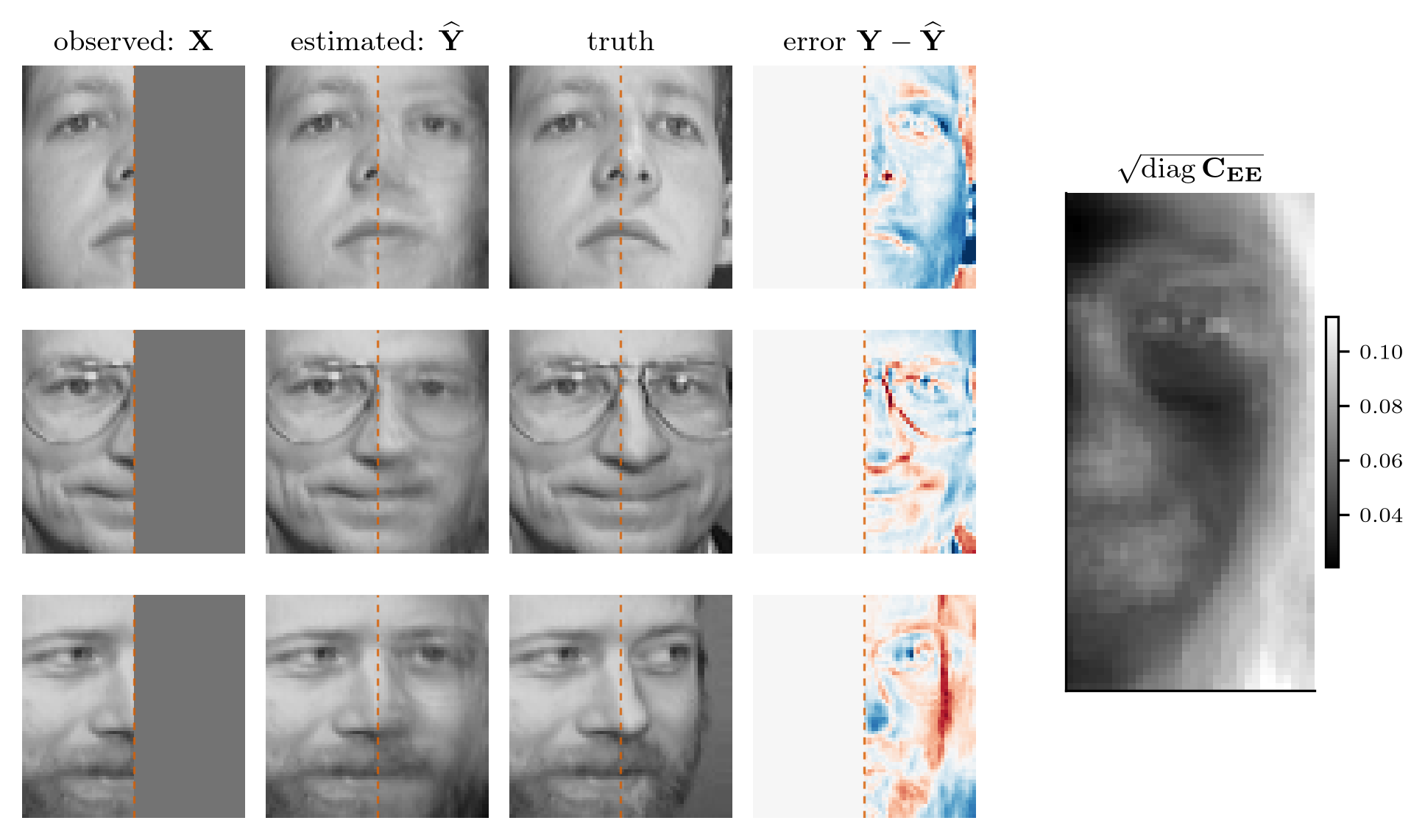
The right half of a face estimated from the left half, with its own error bar per pixel, computed before seeing any face. (Week 5)

Decide whether something is there

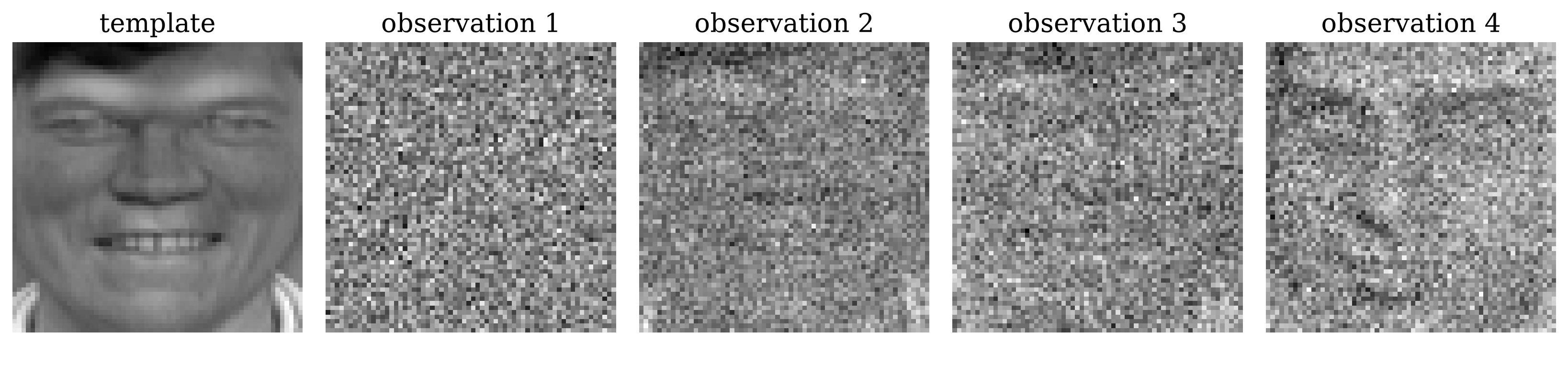
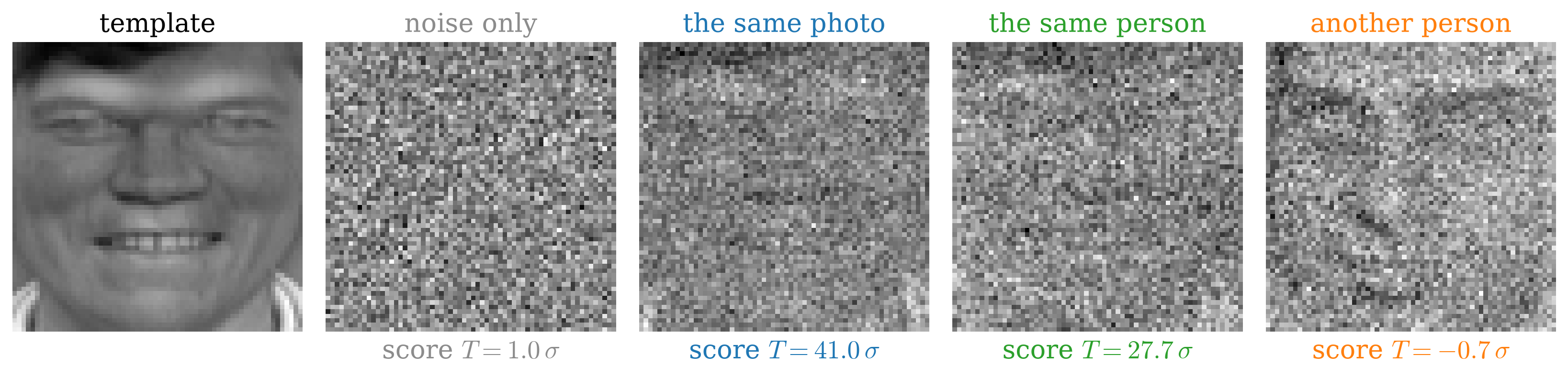
The score is the correlation with the template, in units of its standard deviation under noise alone. Radar, sonar, a wake word, a face in a crowd: correlate with what you expect, compare with a threshold. The matched filter is the best linear detector there is. (Week 6)

Listen in one direction

Eight microphones on a line. A source at angle \(\theta_0\) reaches each one with its own delay \(\tau_i\).

 

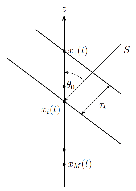
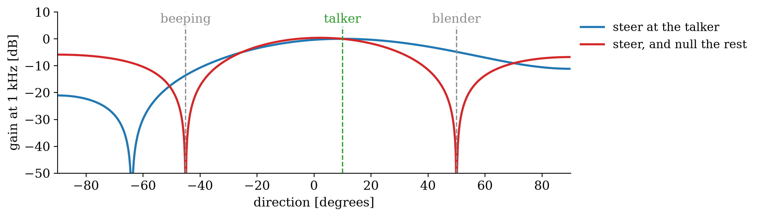
one microphone

steered at the talker

steered, and nulled

A microphone array in a video call, a radio telescope, a 5G base station: steer toward one source and null the others. (Week 6)

Undo a blur

Ground truth, blurred and noisy observation, and the Wiener reconstruction.

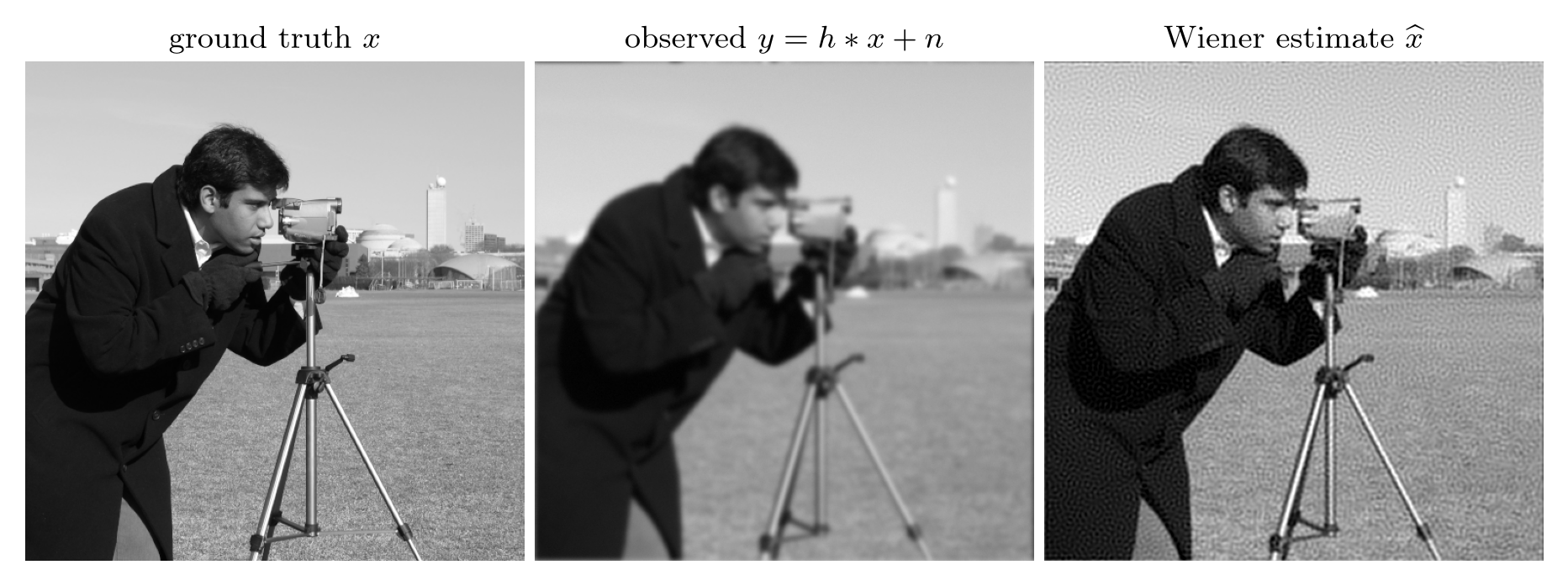
Deblurring is an inverse problem, and naive inversion amplifies the noise without bound. The optimal filter knows which frequencies to trust. (Week 8)

Track something that moves

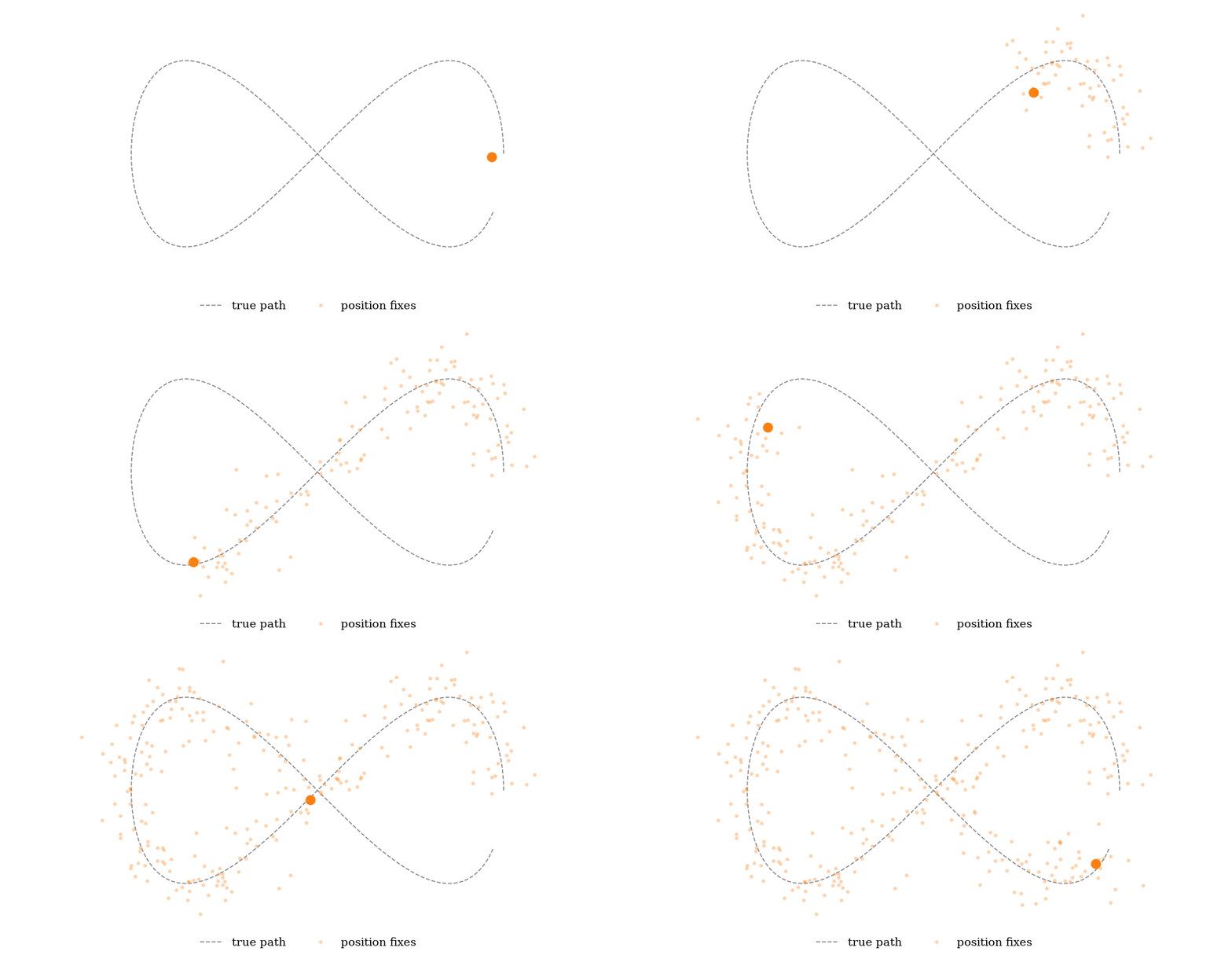
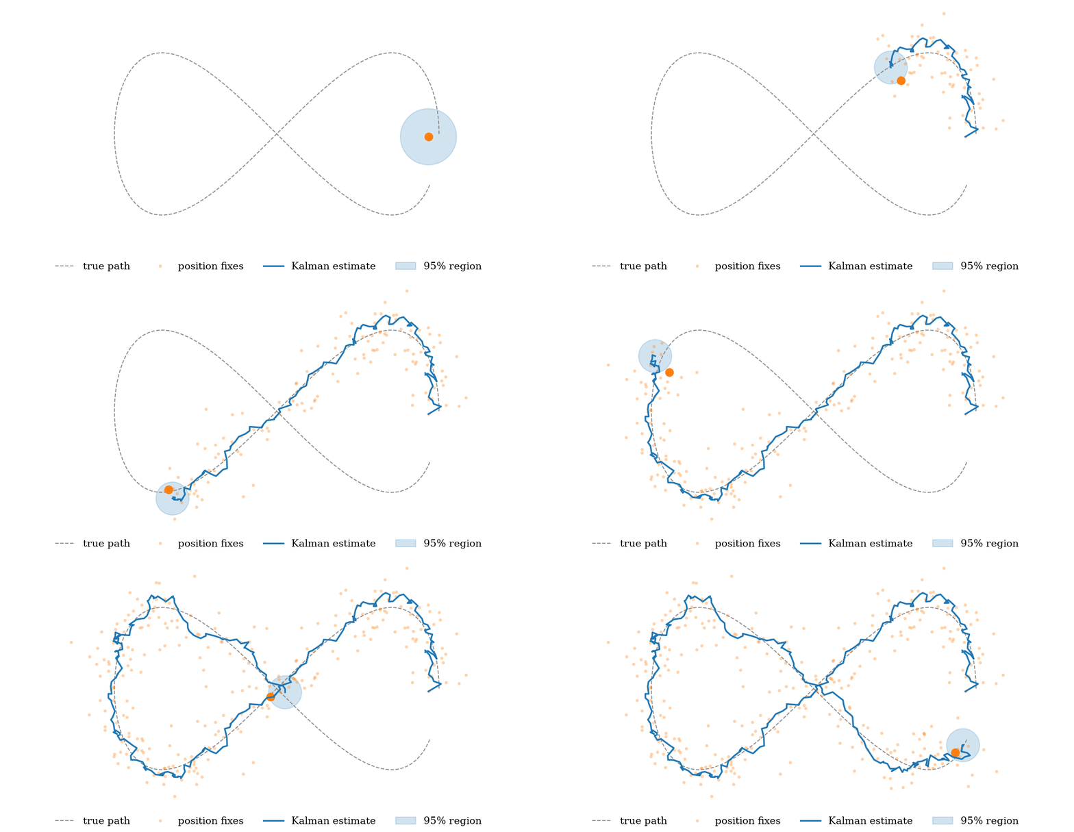
Navigation, a self-driving car, the Apollo guidance computer: predict, measure, correct, repeat. The Kalman filter is how. (Week 9)

Cancel an echo

loudspeaker microphone after cancellation

 

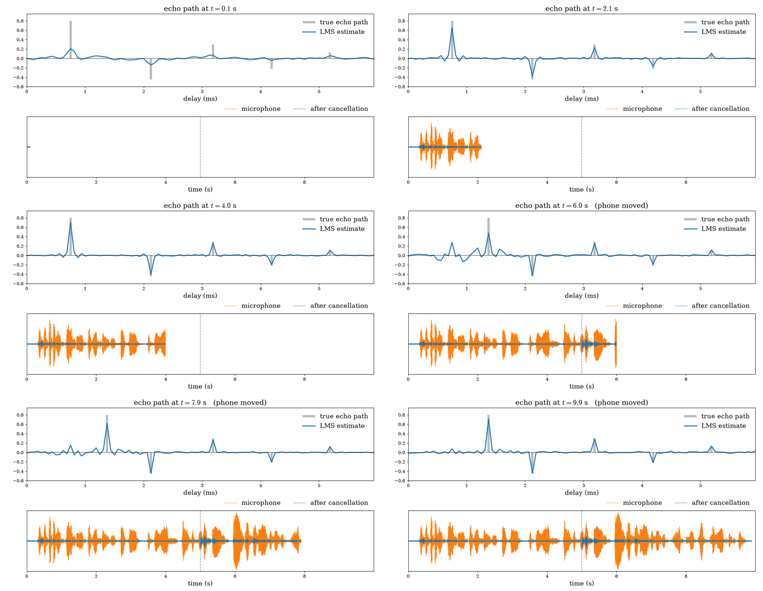
Every phone call on speaker runs an adaptive filter that learns the room while you talk, and keeps learning when you move. (Week 9)

Baked example (figures/code/Echo_LMS_Animation.py): NLMS, 96 taps at 16 kHz, 30 dB SNR. At 5 s the direct sound jumps by 10 samples; the GIF runs in real time, so it can be played alongside the microphone clip. The live version is marimo/live_lms_system_id.py.

The one idea

Seven applications, one right angle

 

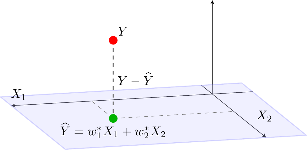
Every one of those systems finds the estimate closest to the truth, among the ones you can build from the data.

“Closest” turns out to be a right angle: the error is orthogonal to everything you observed.

Seven applications, one projection, computed in different spaces.

Concept spiral

 

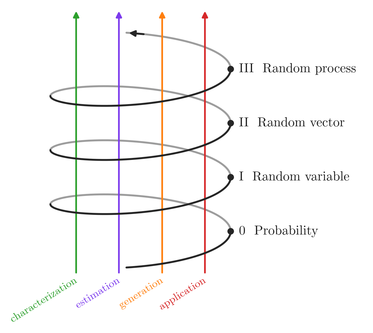
The course climbs one object at a time: a single random variable, then a random vector, then a random process, a vector indexed by time.

At every level the same questions return: characterize the uncertainty, estimate what cannot be seen, generate data from a model, apply it to a real signal.

A technique one level up is the same idea in the notation of a larger object.

Nine weeks

Week		Leaves behind
1	Why Noise Is Gaussian	Sums of many small effects are Gaussian, so two moments suffice
2	Learning a Constant from Data	An estimator is a random variable, with a floor no estimator beats
3	What an Observation Is Worth	The posterior does the work; the conditional mean is the best estimate
4	The Shape of a Random Vector	The covariance matrix is a geometry
5	Estimation Is Projection	The best linear estimate is a right angle
6	One Formula, Four Instruments	Matched filter, beamformer, regularized inverse, fusion
7	When the Index Is Time	Stationarity, the spectrum, white noise through a filter
8	The Wiener Filter	The normal equations become a convolution
9	Estimation That Keeps Up	Predict, then fuse, recursed: Kalman and adaptive filters

Weeks 1–3 are one random variable, 4–6 a random vector, 7–9 a random process: the three turns of the spiral.

What you need, and what you get

Bring

• Signals and systems: convolution, LTI systems, the Fourier transform
• Linear algebra: projections, eigenvalues
• Probability: the basics

Each is revisited where it is needed.

 

Material

• Lecture notes: the reference
• One deck per week: the argument
• Notebooks that run in your browser
• Weekly supplementary sessions for exam preparation

 

Take away

One idea, estimation is projection, and the confidence to recognize it the next time a problem hands you noisy data.