When the Index Is Time

Stationary processes, their spectrum, and white noise through a filter

Three noises

\[ % Number sets \newcommand{\Nat}{\mathbb{N}} \newcommand{\Integer}{\mathbb{Z}} \newcommand{\Real}{\mathbb{R}} \newcommand{\Complex}{\mathbb{C}} % Operators \newcommand{\SNR}{\operatorname{SNR}} \newcommand{\tr}{\operatorname{tr}} \newcommand{\re}{\operatorname{Re}} \newcommand{\im}{\operatorname{Im}} \newcommand{\sign}{\operatorname{sign}} \newcommand{\rect}{\operatorname{rect}} \newcommand{\sinc}{\operatorname{si}} \newcommand{\erf}{\operatorname{erf}} \newcommand{\erfc}{\operatorname{erfc}} \newcommand{\kurt}{\operatorname{kurt}} \newcommand{\diag}{\operatorname{diag}} \newcommand{\MSE}{\operatorname{MSE}} \newcommand{\argmin}{\operatorname*{argmin}} \newcommand{\argmax}{\operatorname*{argmax}} \newcommand{\bias}{\operatorname{bias}} \newcommand{\Bin}{\operatorname{Bin}} % Delimiters \newcommand{\paren}[1]{\left(#1\right)} \newcommand{\bracket}[1]{\left[#1\right]} \newcommand{\set}[1]{\left\{#1\right\}} \newcommand{\abs}[1]{\left\lvert #1 \right\rvert} \newcommand{\norm}[1]{\left\lVert #1 \right\rVert} \newcommand{\ip}[1]{\left\langle #1 \right\rangle} % Notation \newcommand{\dd}{\,\mathrm{d}} \newcommand{\tran}{^{\top}} \newcommand{\conv}{\ast} \newcommand{\conj}{^{*}} \newcommand{\herm}{^{\mathsf{H}}} \newcommand{\opt}{^{\star}} % Expectation and variance % \newcommand{\E}[1]{\mathbb{E}\!\left[#1\right]} \newcommand{\E}[2][]{\mathbb{E}_{#1}\!\left[#2\right]} \newcommand{\Var}[1]{\mathbb{V}\!\left[#1\right]} % Distributions \newcommand{\Gauss}{\mathcal{N}} \newcommand{\Uniform}{\mathcal{U}} \newcommand{\FT}{\mathcal{F}} % Probability \newcommand{\Prob}[1]{\mathbb{P}\!\left(#1\right)} % Misc \newcommand{\bsy}[1]{\boldsymbol{#1}} \newcommand{\calR}{\mathcal{R}} \newcommand{\calC}{\mathcal{C}} \]

Same power, different sound

Three recordings, each with the same variance at every instant, and each Gaussian:

Hiss, rumble, a thin sizzle: identical histograms. What tells them apart is how each sample relates to its neighbors.

A signal is a random vector that never ends: the Fourier transform does for it what the eigenvectors did for a face.

Left: white noise. Middle: white noise through a one-pole low-pass (pole at 0.97). Right: white noise through a first difference. All three are normalized to unit variance.

The plan for the week

Describing a process. The autocorrelation, stationarity, white noise, and when one recording can stand in for all of them (ergodicity).

The spectrum. The power spectral density, what a filter does to it, and why every stationary process is white noise through a filter. Then back to a finite window, where the Fourier basis turns out to be the KLT.

In the notes Definition of a Random Process · Distributions and Expectations · Stationarity · Ergodicity · Power Spectral Density · LTI Systems and WSS Processes · Coloring, Whitening, and Spectral Factorization · The Finite Window

A random vector that never ends

Two ways to read a process

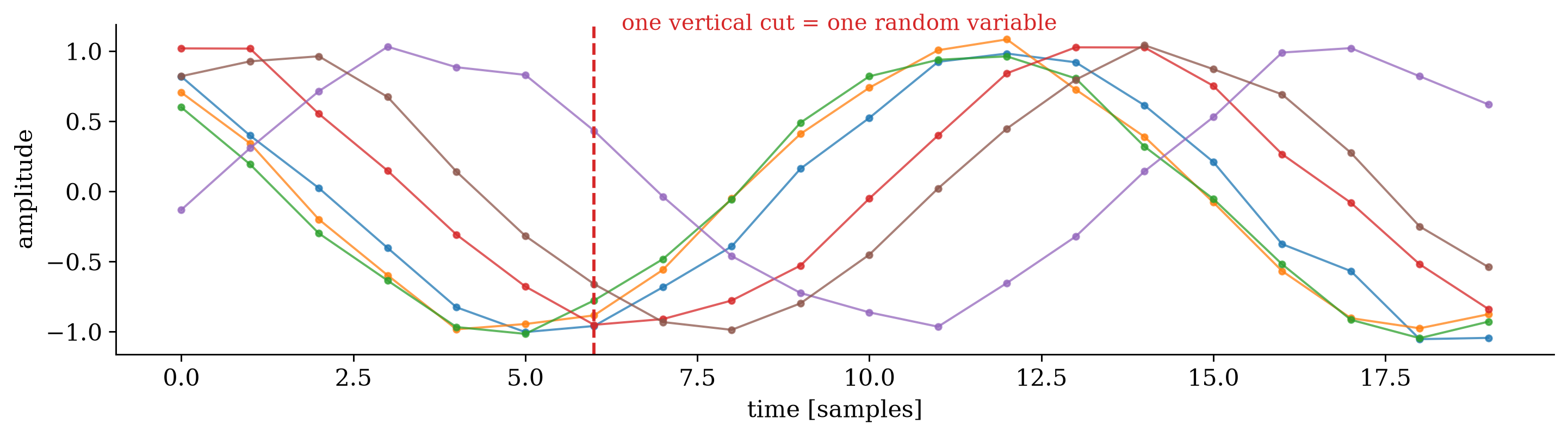
A random process assigns a whole sequence \(X[\eta,k]\) to each outcome \(\eta\).

Down the ensemble: one random variable per time instant. Along time: one realization, the recording you actually have.

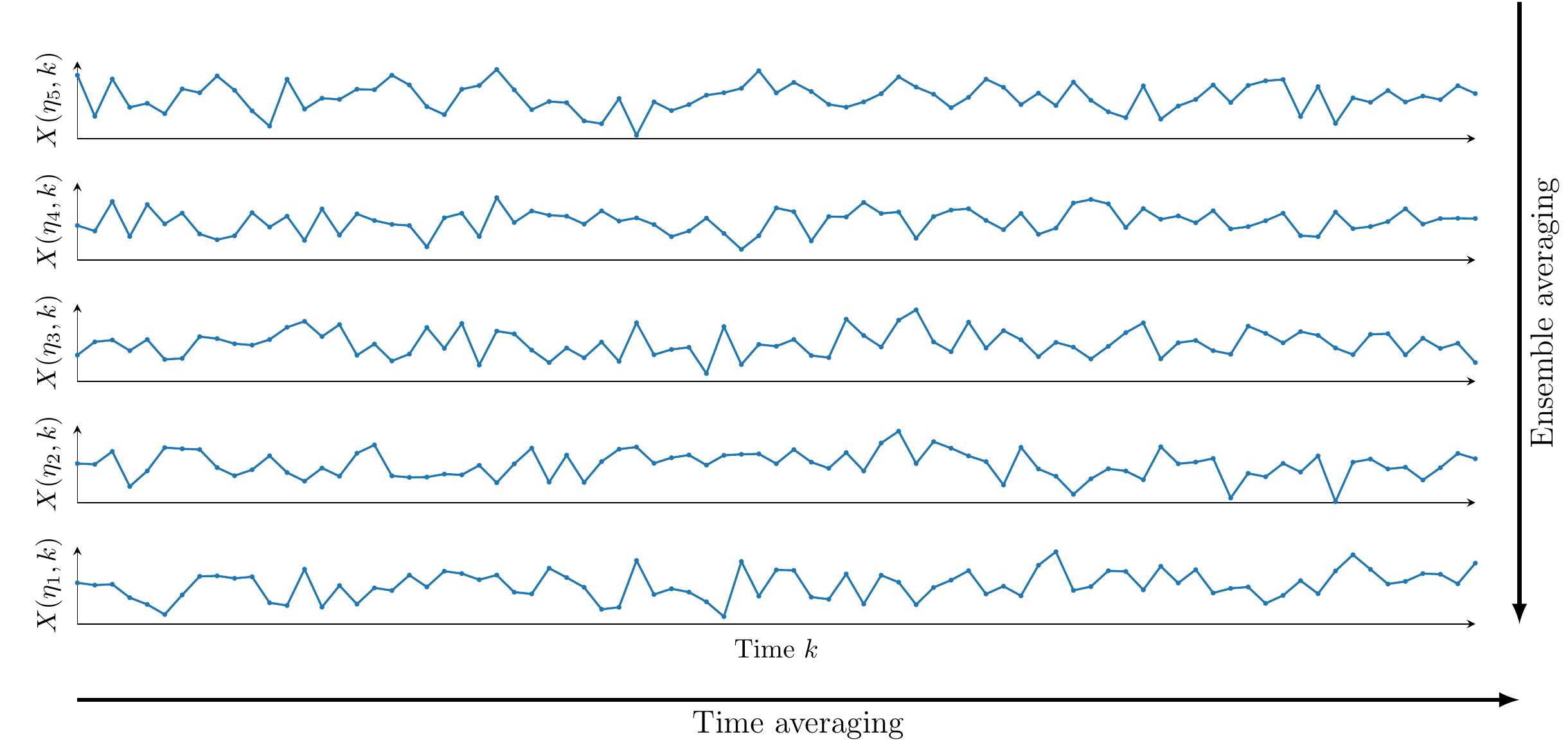
Randomness chosen once, played out in time

Figure 1: Six realizations of X[k] = sin(ωk + Φ) + W[k] with Φ uniform: each realization is one draw of the phase.

Its second-order description is the autocorrelation \(R_{XX}[k_1,k_2]=\E{X[k_1]\,X\conj[k_2]}\): the correlation matrix of the random-vector week, with infinitely many rows.

Two moments, now functions of time

Moments of a process \[m_X[k]=\E{X[k]},\qquad R_{XX}[k_1,k_2]=\E{X[k_1]X\conj[k_2]},\qquad R_{XY}[k_1,k_2]=\E{X[k_1]Y\conj[k_2]} .\]

The arithmetic of the random-vector week carries over line by line: correlations of sums add up their cross terms, and delaying a process delays its correlation, \(Y[k]=X[k-\kappa_0]\Rightarrow R_{XY}[k_1,k_2]=R_{XX}[k_1,k_2-\kappa_0]\).

The same rule names every correlation: first index plain, second conjugated. Swapping the subscripts is taking the adjoint.

Three processes with no memory

Gaussian, uniform and \(\pm1\) noise of equal power, and their first-order densities.

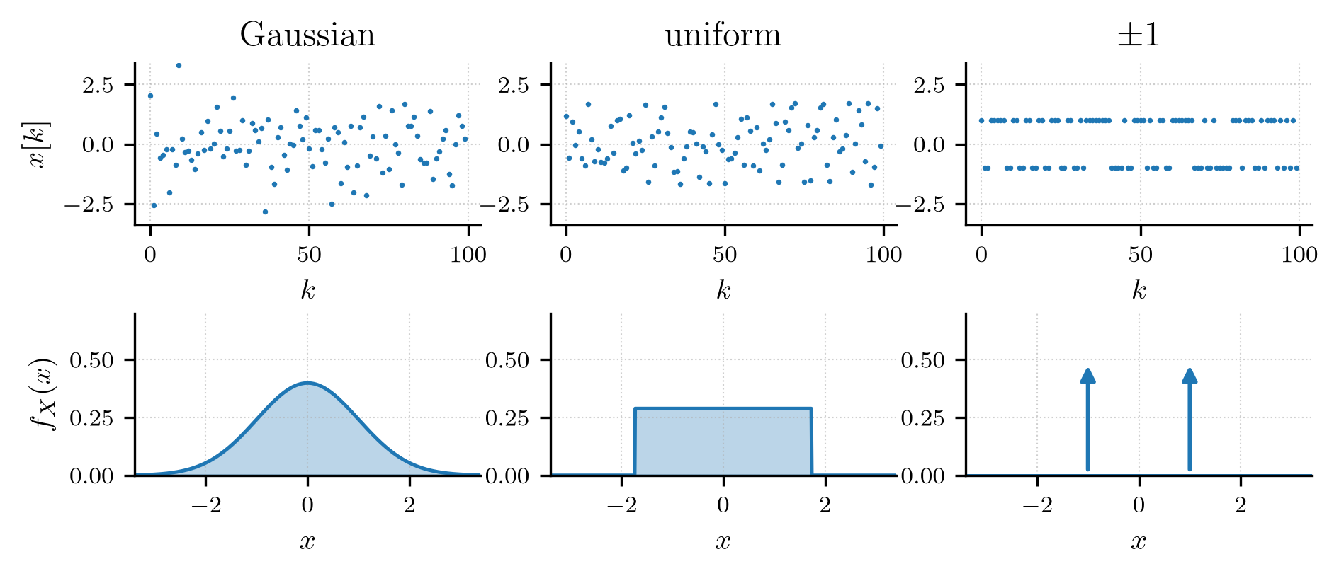
Three different laws and one identical autocorrelation, \(\sigma^2\delta[\kappa]\). Everything second-order in this course sees these three as the same process.

A process that remembers everything

The random walk \(X[k]=X[k-1]+W[k]\): realizations inside the \(\pm\sqrt k\,\sigma\) envelope, and the ensemble cut at several instants.

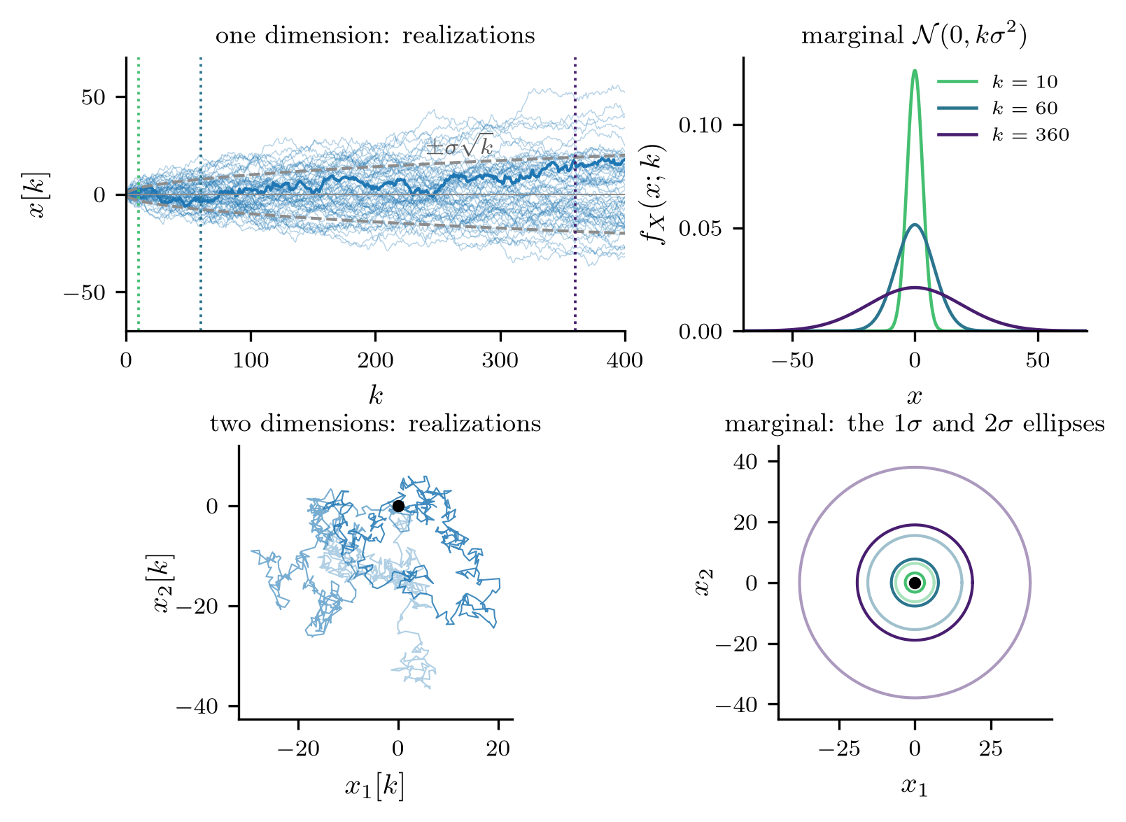
The variance grows like \(k\) and the process never settles: the law at time \(k\) depends on \(k\). For most of signal processing we want the opposite.

A multiplicative walk

Multiplying instead of adding: the mean rises, the median stays at one, the mode falls; the log-normal marginal at three instants.

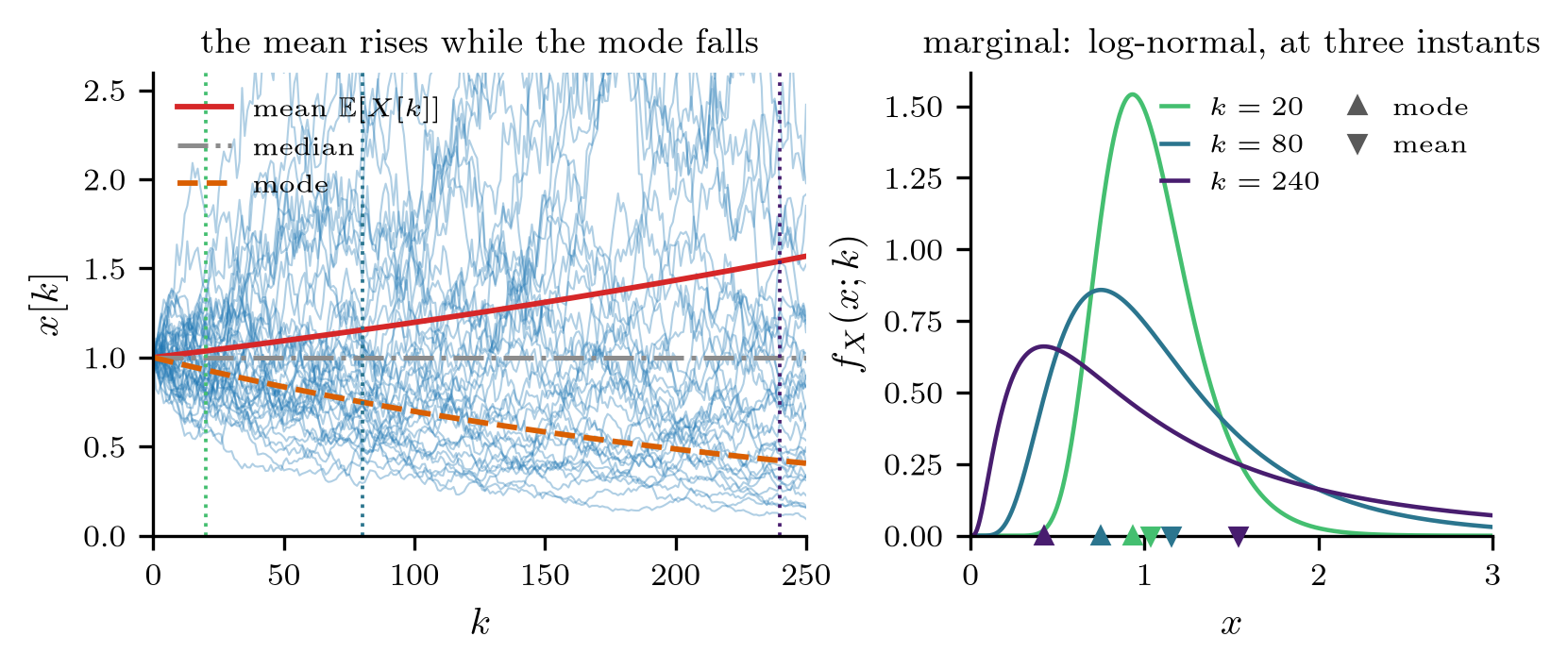
Mean, median and mode drift apart as time goes on. A typical realization tells you very little about the ensemble mean: a warning worth keeping in mind for ergodicity.

Neighbors in real sound

Figure 2: The /ks/ of a recorded word. Left: the waveform. Right: the joint histogram of consecutive samples.

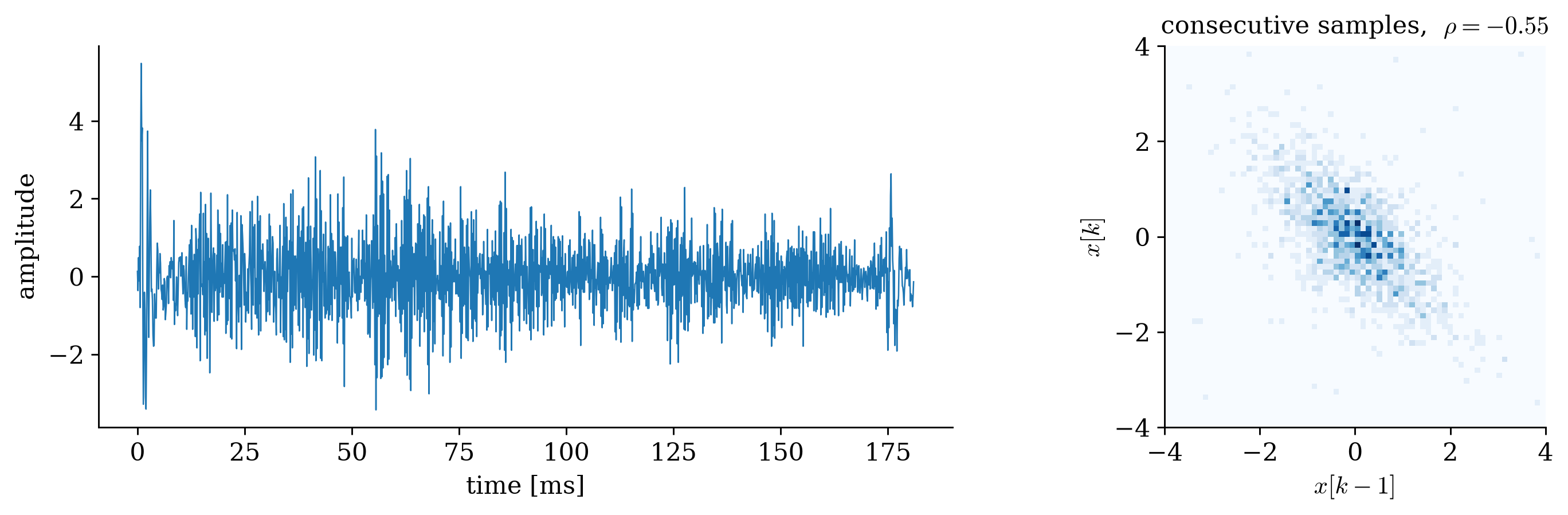
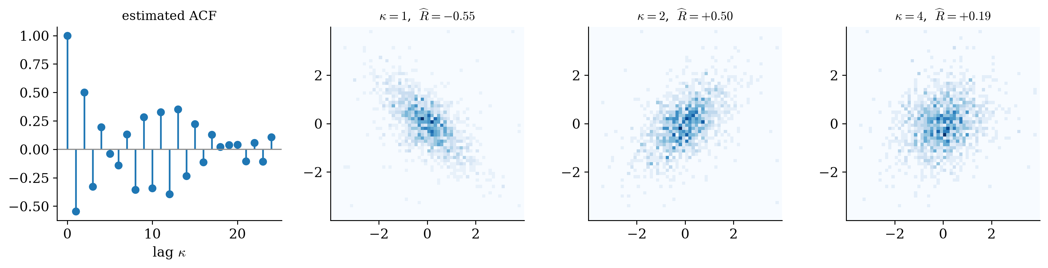
The marginal alone says “noise”. The joint law of two consecutive samples is tilted: adjacent samples are negatively correlated, the time-domain signature of a hissing, high-frequency sound.

Stationarity

Randomize the phase

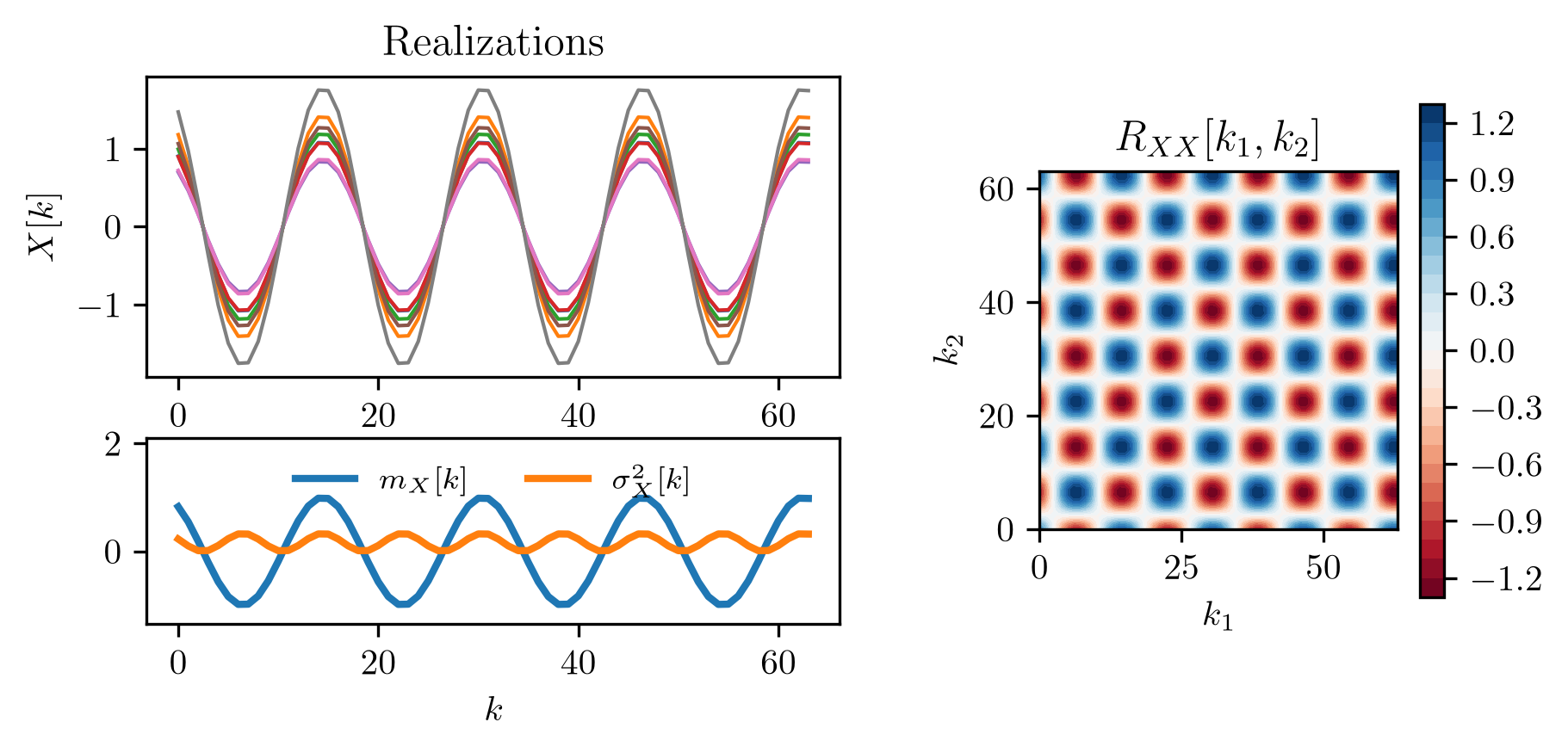
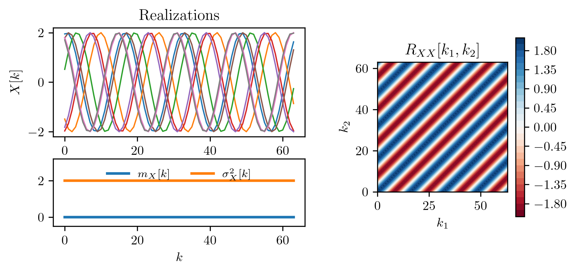
Wide-sense stationary (WSS) Constant mean, and an autocorrelation that depends only on the lag: \(R_{XX}[k+\kappa,k]=R_{XX}[\kappa]\). Strict-sense stationary: every joint law is shift-invariant.

Not knowing when you started listening is what makes a process stationary.

Strict, wide, and the Gaussian coincidence

Strict and wide sense

• Strict implies wide: if every law is shift-invariant, so are the first two moments. The converse fails in general.

• For Gaussian processes it holds: their laws are fixed by mean and covariance alone.

The same collapse that made uncorrelated equal independent for Gaussian vectors. This course lives in the wide sense: first and second moments are what linear estimation needs.

What an autocorrelation must satisfy

Properties of a WSS autocorrelation \[R_{XX}[\kappa]=R_{XX}\conj[-\kappa],\qquad R_{XX}[0]=\E{\abs{X[k]}^2}\ge\abs{R_{XX}[\kappa]},\] and every finite window of lags forms a positive semidefinite matrix.

The second is Cauchy–Schwarz on \(X[k+\kappa]\) and \(X[k]\); the third says that no linear combination of samples can have negative power.

The peak at lag zero is what lets a cross-correlation locate a delay.

Correlation finds a delay

Two microphones hear one source, the second farther away: \(Y[k]=X[k-\kappa_0]+N[k]\).

Left: the two recordings; the delay is invisible. Right: the cross-correlation peaks at \(\kappa_0\).

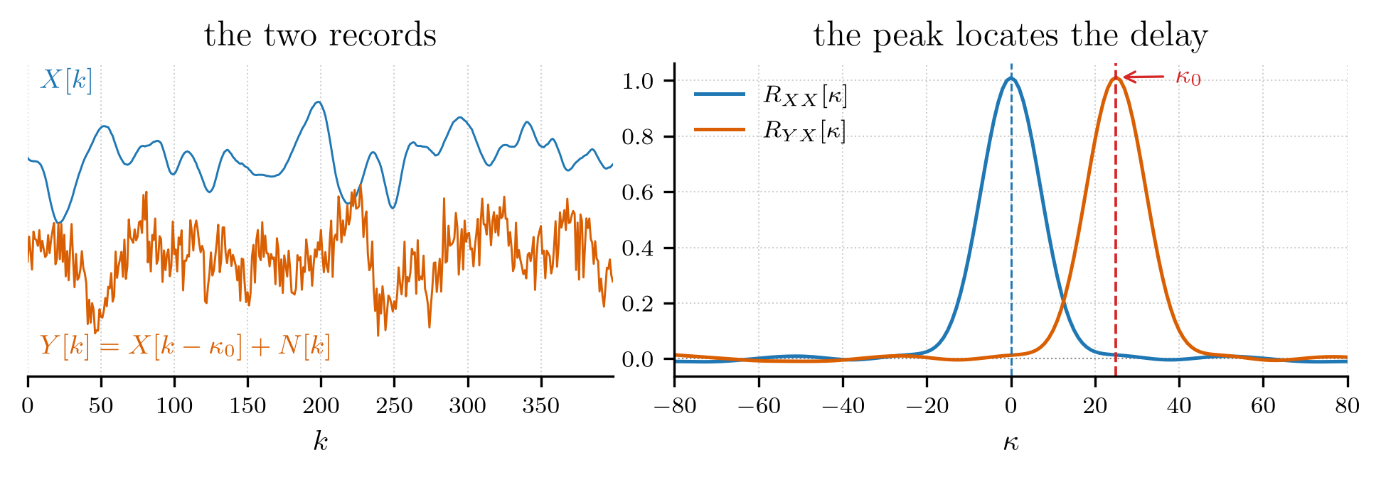
The noise drops out of the cross-correlation and only the shifted \(R_{XX}[\kappa-\kappa_0]\) remains, peaked at \(\kappa_0\) because \(\abs{R_{XX}}\) is largest at zero lag. This is how sound sources and radar echoes are located.

A sinusoid in noise

A sinusoid buried in noise: one realization, in which the periodicity is not apparent, and its autocorrelation, where the noise is one spike at lag zero and the tone a slow cosine.

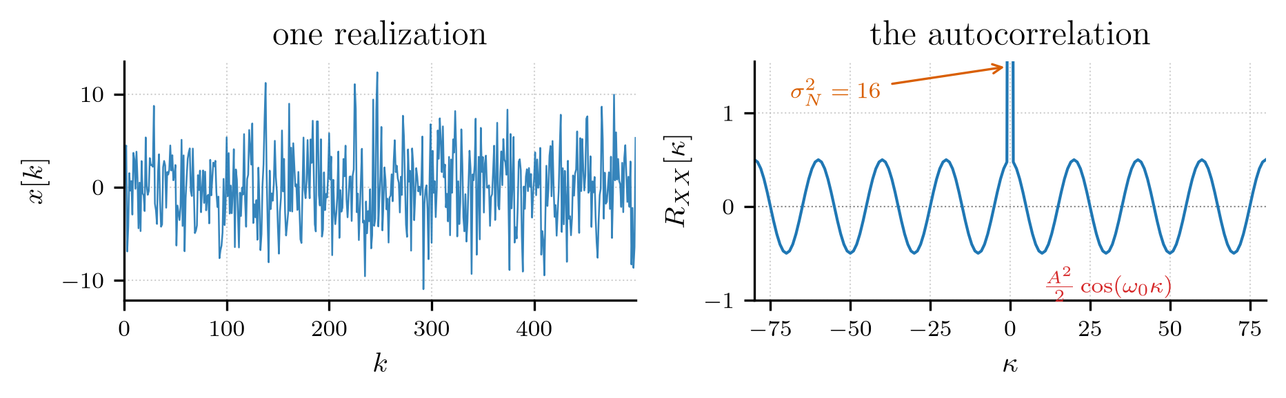
Second-order statistics find what the trace hides: the tone survives at every lag, the noise only at lag zero.

White noise

White noise \(R_{XX}[\kappa]=\sigma^2\,\delta[\kappa]\): distinct instants uncorrelated, equal power, a process whose covariance matrix is the identity. Strictly white: distinct instants independent.

\(X[k]=W[k]W[k-1]\): white, since neighbors are uncorrelated, yet the joint density of neighbors is not a product.

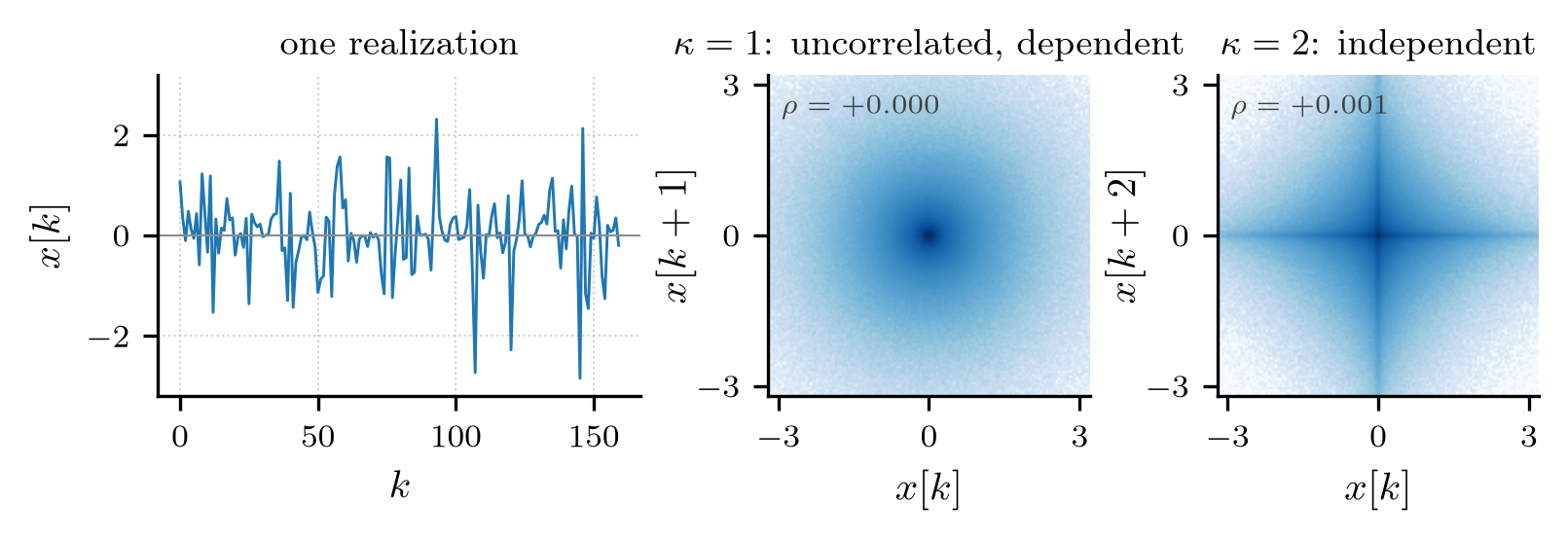
Whiteness is a second-order statement. Only for a Gaussian process does white mean independent.

White is not unpredictable

A tone of random frequency and phase: each realization is a pure cosine, and across the ensemble the process is white.

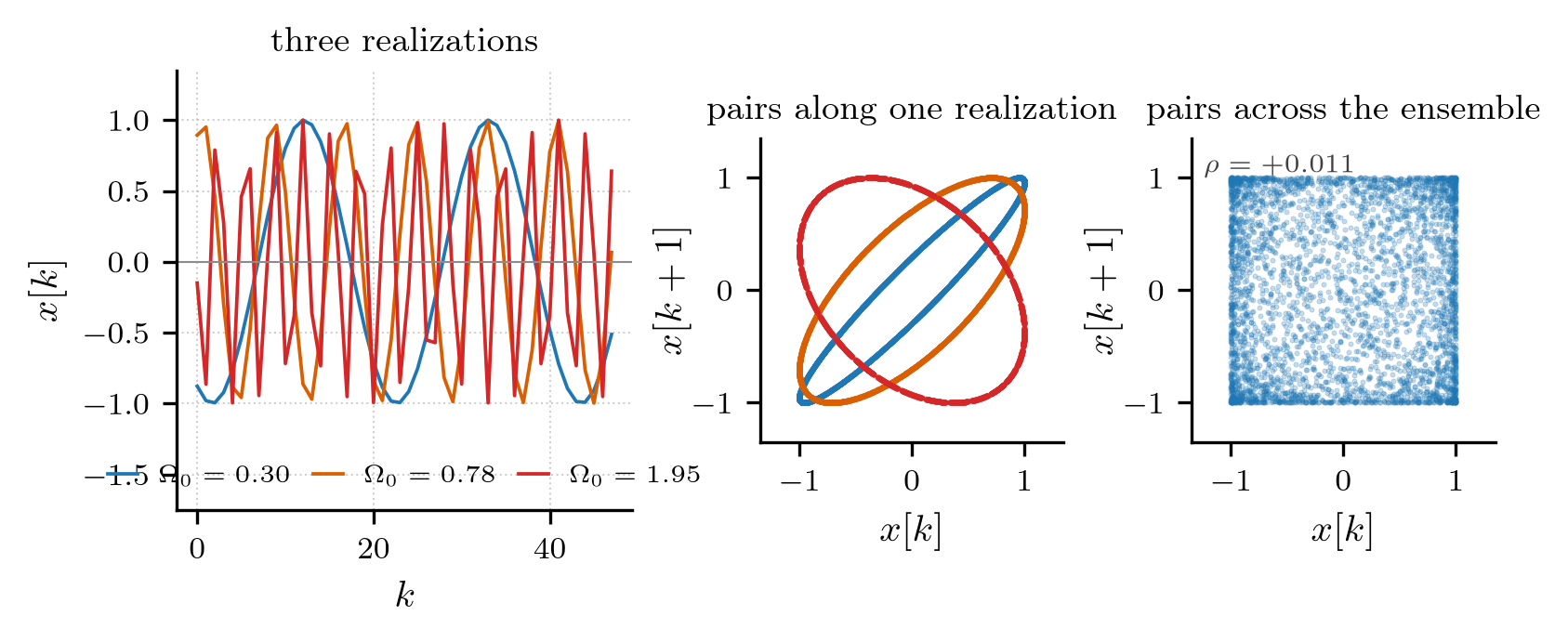
Every realization obeys \(X[k+1]=2\cos(\Omega_0)X[k]-X[k-1]\). Three samples reveal the frequency, and everything after is predicted exactly.

Whiteness rules out linear predictability, not predictability. The best linear predictor of this process is zero; a nonlinear one is perfect.

Three independent properties

Figure 3: White and stationary; white but not stationary (the variance decays); white and stationary but not Gaussian.

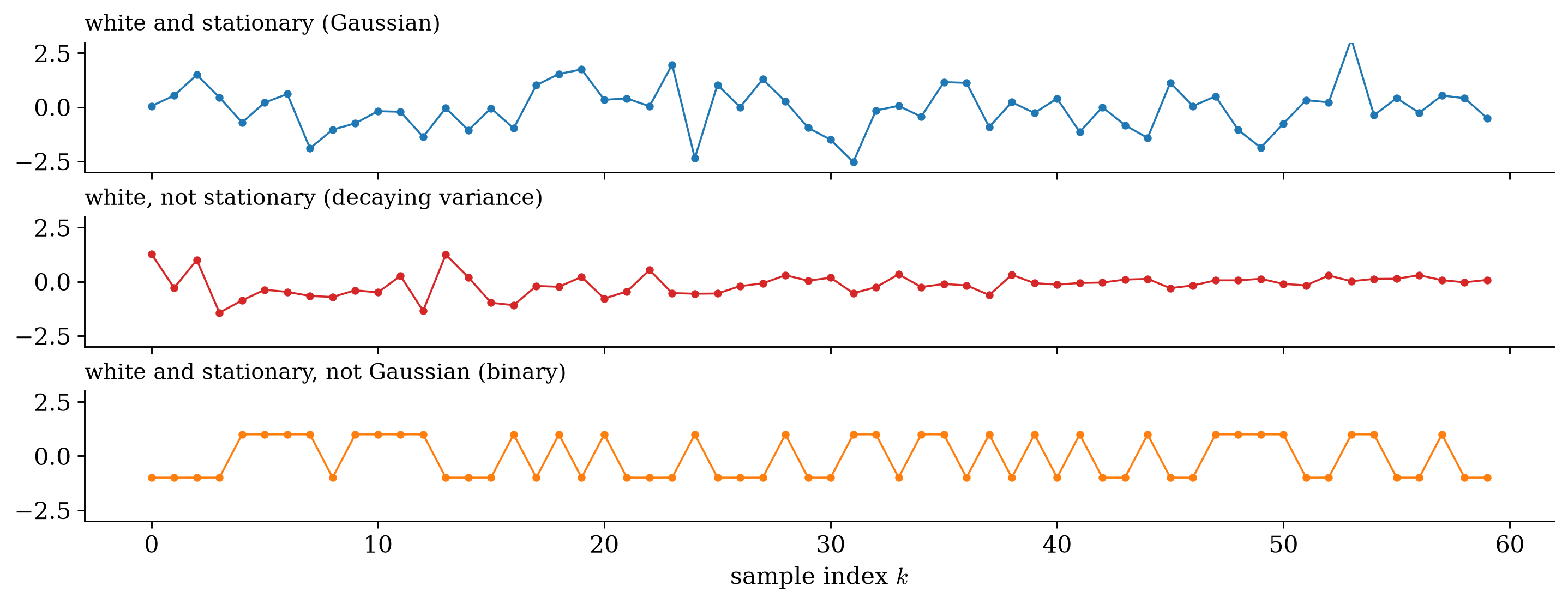
“White” is about correlation across time, “stationary” about drift of the statistics, “Gaussian” about the shape of the law. Name which one a claim is about.

One record for the ensemble

Ergodicity

You have one recording, not an ensemble. Time averages must stand in for expectations:

Ergodic in the mean and in correlation \[\frac{1}{2K+1}\sum_{k=-K}^{K}x[k]\to m_X,\qquad \frac{1}{2K+1}\sum_{k=-K}^{K}x[k+\kappa]\,x\conj[k]\to R_{XX}[\kappa] .\]

It works when correlations die out: a time average is a sample mean of correlated terms, and its variance still shrinks as long as \(\sum_\kappa\abs{C_{XX}[\kappa]}<\infty\).

Seen directly

Figure 4: A stable AR(1) process. Left: the ensemble average over 400 realizations at each time. Right: the time average along four single realizations.

Why the time average converges

The time average over \(2K+1\) samples is a sample mean of correlated terms, so its variance keeps the cross terms:

Variance of the time average \[\Var{\bar x_K}=\frac{1}{2K+1}\sum_{\abs\kappa\le2K}\paren{1-\frac{\abs\kappa}{2K+1}}C_{XX}[\kappa] \;\approx\;\frac{1}{2K+1}\sum_\kappa C_{XX}[\kappa] .\]

If the covariance is summable this falls like \(1/K\): the effective sample size of correlated averaging, now along time. A process whose correlation never dies out has no such guarantee.

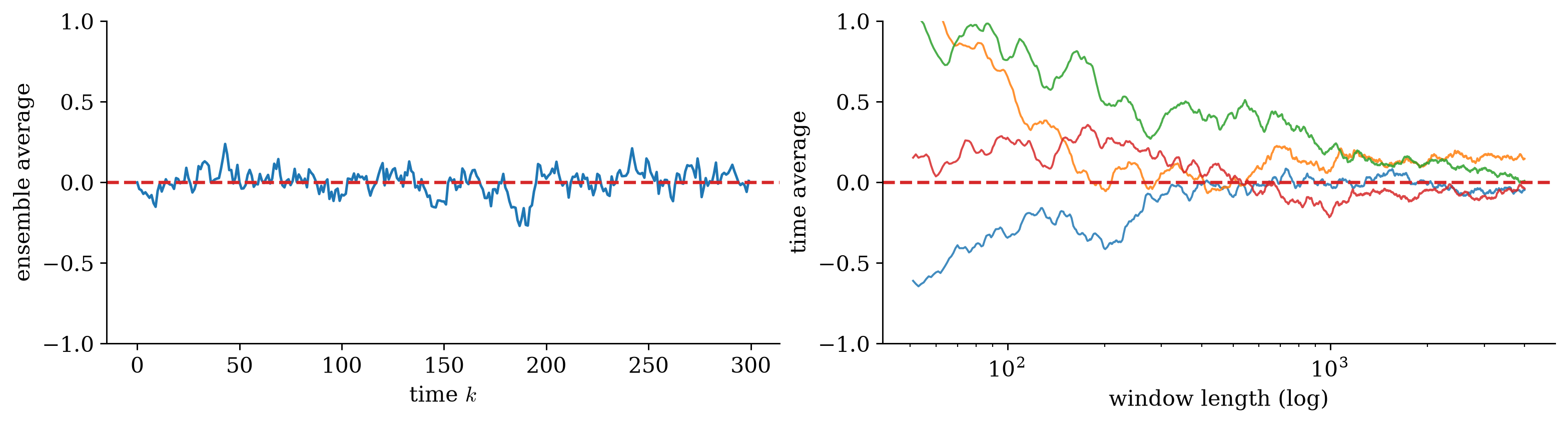
How fast one record settles

Figure 5: Variance of the time average over K samples of a unit-variance AR(1) process, for three pole values, against the iid rate 1/K.

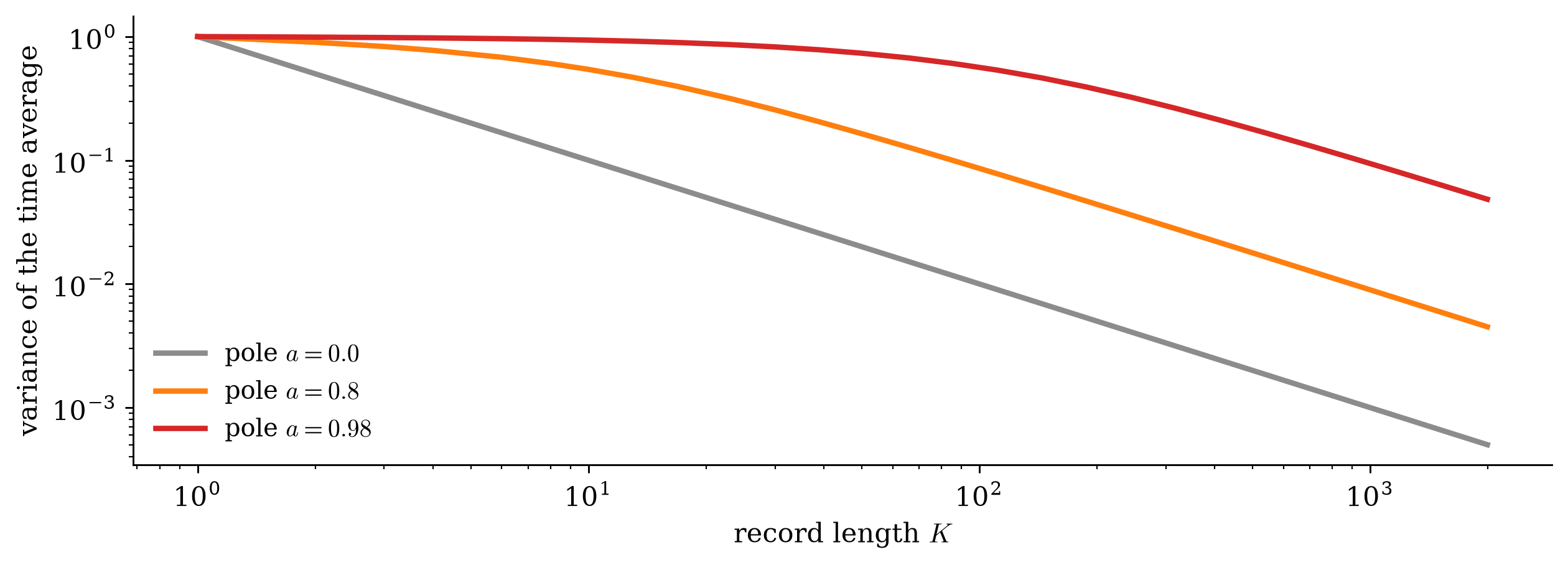
Every curve falls like \(1/K\) eventually; strong correlation only delays it. At \(a=0.98\) a record must be about a hundred times longer than for white noise to be worth the same.

Correlation in hardware

Delay, multiply, average: the correlation function falls out of a structure with no expectation in it anywhere.

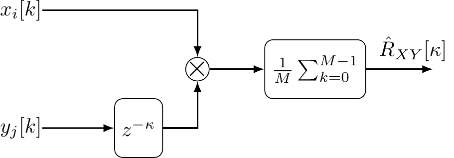
\(R_{XX}[\kappa]\) is defined over an ensemble no laboratory has. What is built is a delay line, a multiplier and an integrator, and ergodicity is the entire justification for calling its output \(R_{XX}[\kappa]\).

One recording, read as a process

Figure 6: The /ks/ segment. Left: the time-averaged autocorrelation estimate. Right: the joint law of (x[k], x[k−κ]) at three lags.

Every number came from one recording, averaged along time, and is read as a property of the process.

When it fails

Pólya’s urn: each realization converges, but to its own limit.

A process constant along time: stationary, and every time average is just its own level.

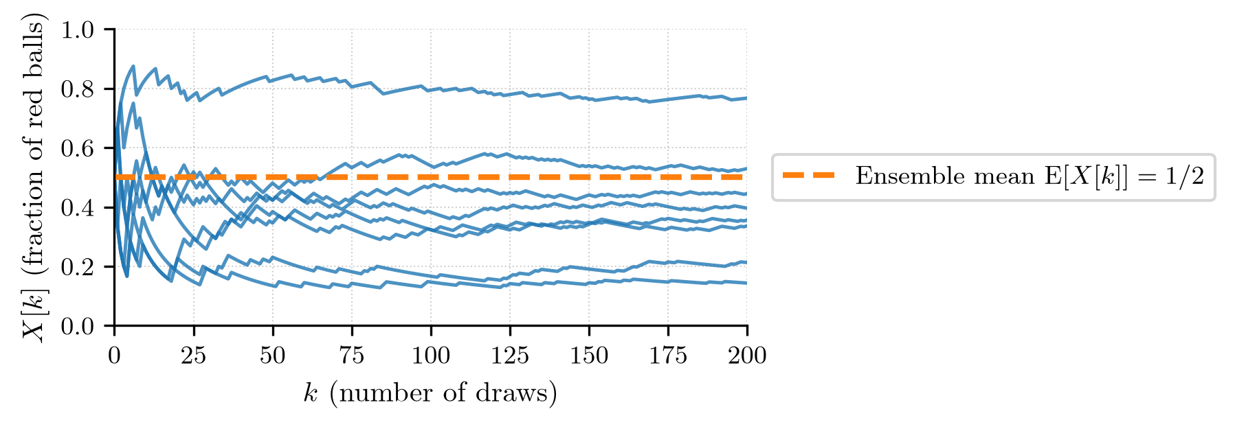
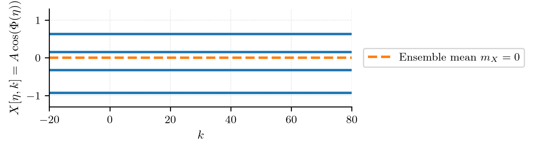
Stationarity and ergodicity are independent properties. A parameter drawn once per realization (a per-device offset, a per-session gain) is never averaged out by time.

The spectrum

The power spectral density

Power spectral density The limit of the expected periodogram, \[S_{XX}(e^{j\Omega})=\lim_{N\to\infty}\frac{1}{2N+1}\E{\abs{X_N(e^{j\Omega})}^2}.\]

Wiener–Khinchin \(S_{XX}(e^{j\Omega})=\sum_\kappa R_{XX}[\kappa]\,e^{-j\Omega\kappa}\), the Fourier transform of the autocorrelation.

White noise has a flat spectrum, which is where the name comes from. The expectation must come before the limit: a single periodogram never settles down.

Why the expectation comes first

Figure 7: White noise of unit power: one periodogram of 1024 samples (grey), the average of 32 periodograms (blue), and the true PSD (red).

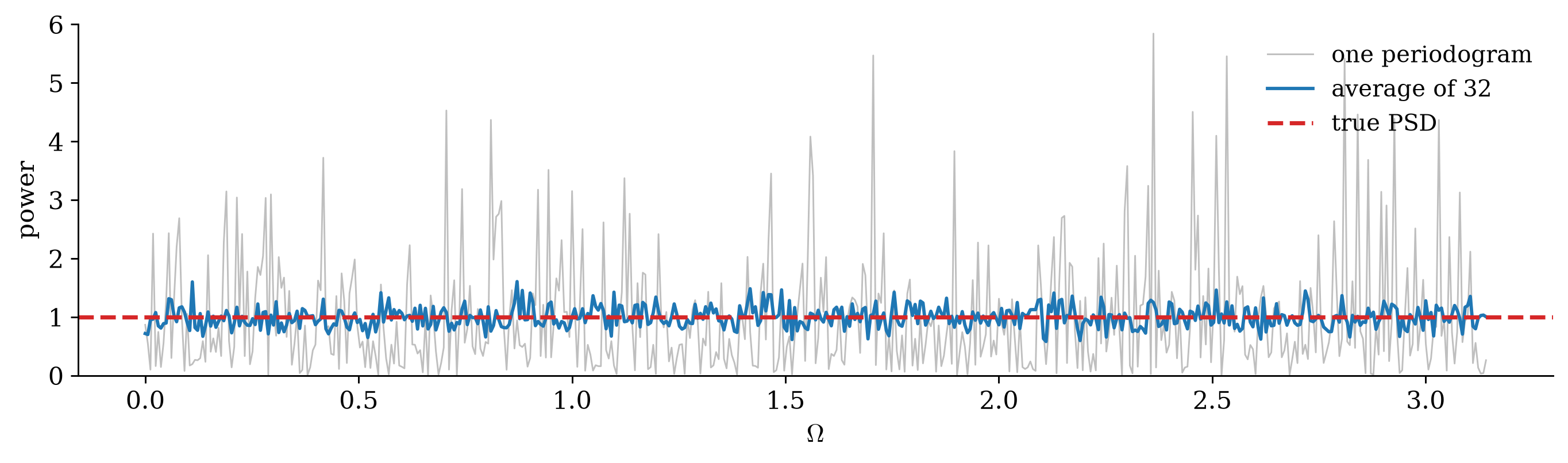
A longer record gives more frequencies, not steadier ones. The spectrum belongs to the ensemble, which is why the definition takes the expectation before the limit.

It really is a density of power

Power is the area under the PSD \[\E{\abs{X[k]}^2}=R_{XX}[0]=\frac{1}{2\pi}\int_{-\pi}^{\pi}S_{XX}(e^{j\Omega})\dd\Omega .\]

Pass the process through a narrow bandpass around \(\Omega_0\): the output power is \(S_{XX}(e^{j\Omega_0})\) times the bandwidth. That is also why \(S_{XX}\ge0\): a power cannot be negative.

It really is a density of power

A sinusoid in noise, read in frequency: the noise is a flat floor, the tone a pair of lines.

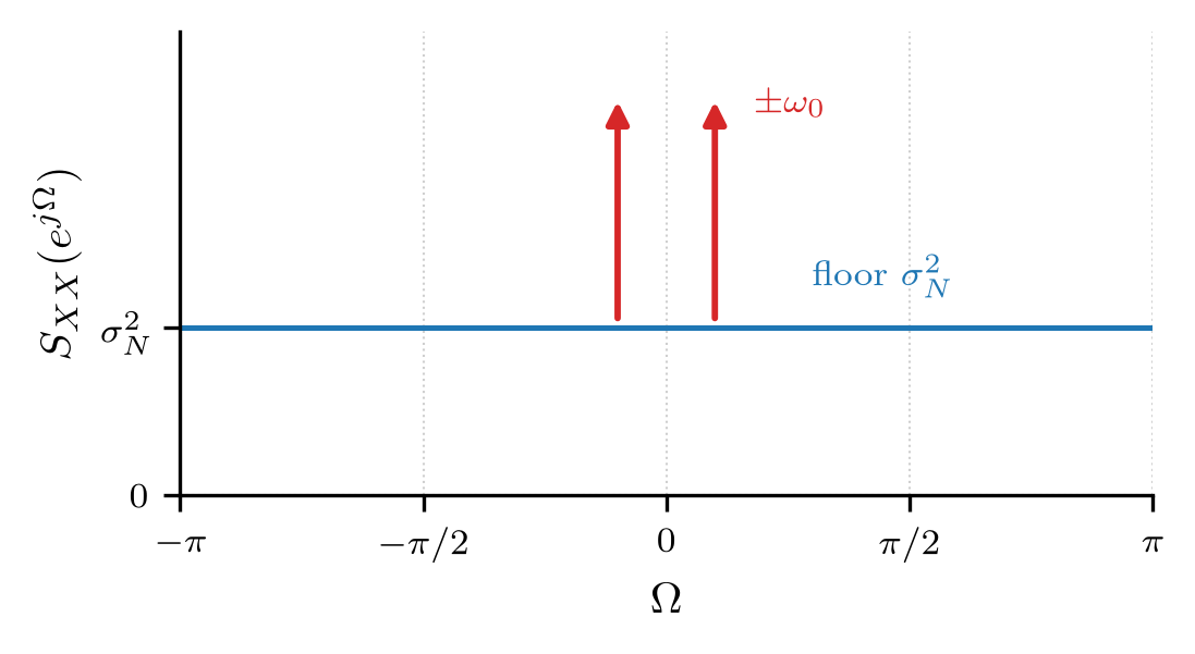
What is concentrated in one domain is spread in the other. Detecting a tone in noise is easy in frequency and hard in time.

The spectrum of a real sound

Figure 8: The /ks/ segment: its estimated autocorrelation, and its spectrum.

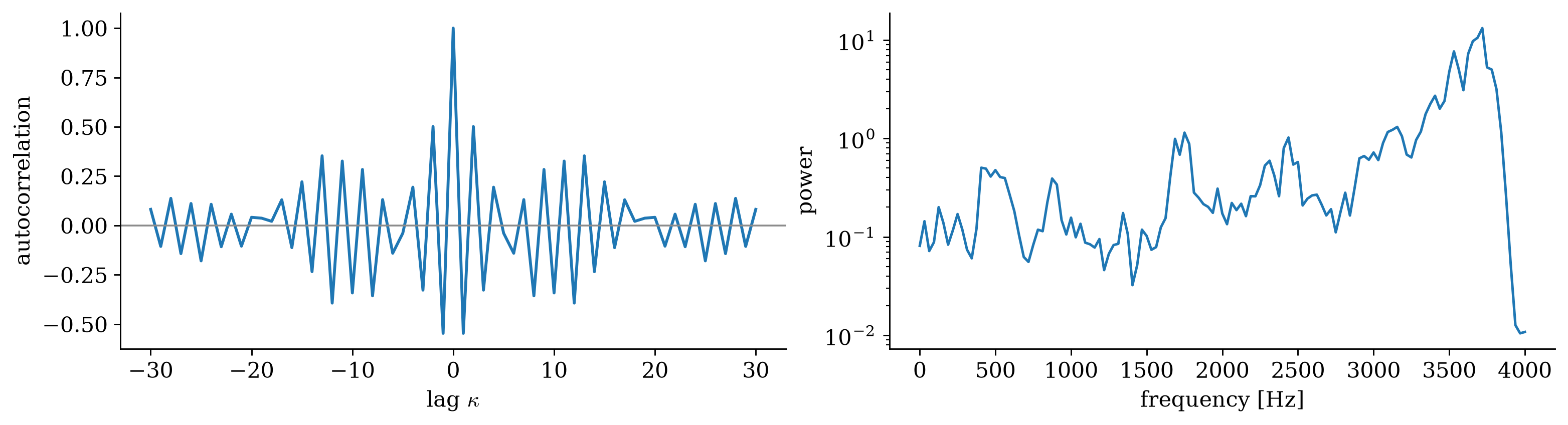
The sign alternation of the autocorrelation and the rise of the spectrum with frequency are one fact, read in two domains.

The delay, read in frequency

The delay measurement in frequency: the cross-spectrum magnitude (the source spectrum), its phase (a straight line of slope \(-\kappa_0\)), and the coherence, which says where the phase can be trusted.

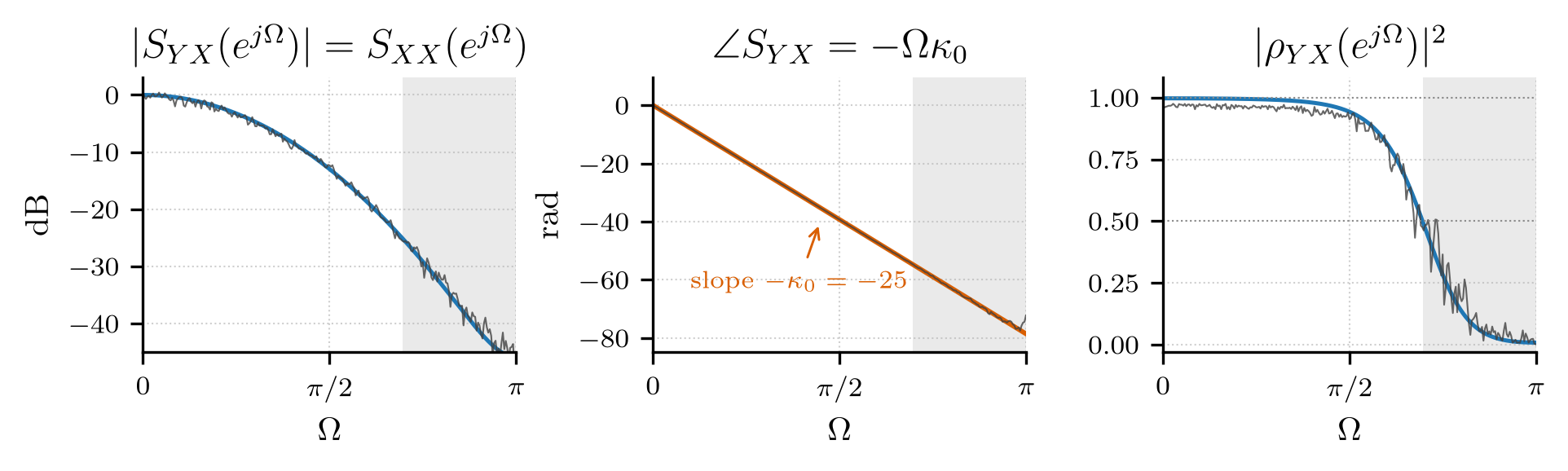
A delay is a linear phase. The coherence \(\abs{S_{YX}}^2/(S_{XX}S_{YY})\) is a squared correlation coefficient, one frequency at a time: where it collapses, the noise has won and the phase is garbage.

What a filter does

White noise through a filter

WSS through an LTI filter For a stable filter \(h\) with frequency response \(H\), \(Y=h*X\) is WSS again, with \[R_{YX}=h*R_{XX},\qquad S_{YX}=H\,S_{XX},\qquad S_{YY}=\abs{H}^2\,S_{XX}.\]

White noise through a filter

White noise through a filter: input and output, and their spectra.

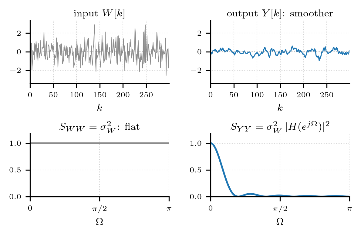
The process version of \(\mathbf C_{\mathbf{YY}}=\mathbf A\mathbf C_{\mathbf{XX}}\mathbf A\herm\): a filter reshapes the spectrum by \(\abs{H}^2\). That is what you heard at the start.

→ Demo: AR(1) autocorrelation and spectrum

Filtering also Gaussianizes

Figure 9: A binary ±1 input through a long low-pass filter: each output sample is a weighted sum of many independent inputs.

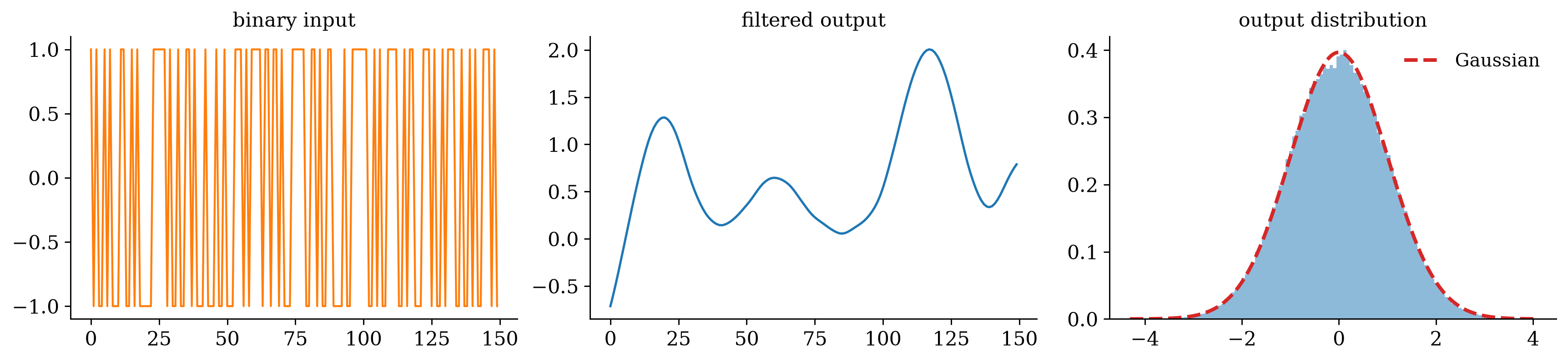
A filter colors, which is the second-order statement \(\abs{H}^2S_{XX}\). A filter also Gaussianizes, which is a statement about the whole law: the central limit theorem of the first week, at work inside every filter.

Every process is white noise through a filter

Wold decomposition Every WSS process is the sum of a causal filtering of its own white innovations and a part that is perfectly predictable from its past.

So the spectrum factors, \(S_{XX}=\sigma_W^2\abs{H}^2\), with \(H\) causal and minimum phase, as long as \(\int\abs{\ln S_{XX}}\dd\Omega<\infty\) (Paley–Wiener). Then \(1/H\) is causal too, and it whitens: it recovers the innovations.

A spectrum that vanishes on a whole band fails Paley–Wiener: such a process is linearly deterministic, with nothing left to whiten.

Constructing the causal factor

Spectral factorization through the cepstrum: take the log of the spectrum, transform to the cepstrum, keep the causal half, exponentiate.

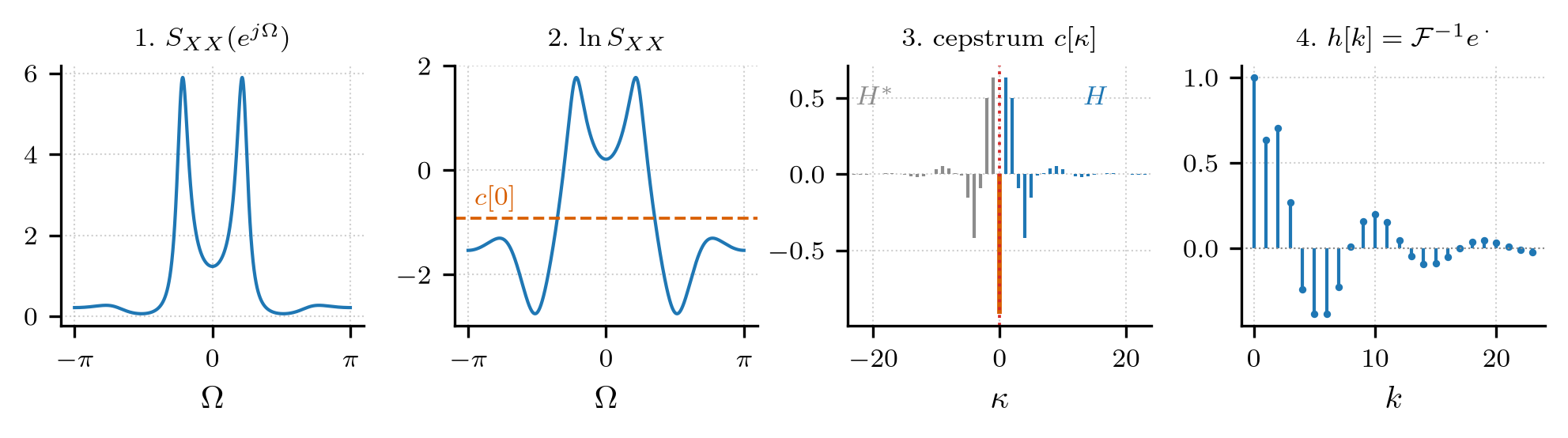
The logarithm turns the product \(\sigma_W^2HH\conj\) into a sum, and causality becomes “keep the right half”. The innovation power \(\sigma_W^2\) is the geometric mean of the spectrum.

→ Demo: whitening temperature records by spectral factorization

Three whiteners, one level up

random vector	stationary process
Cholesky \(\mathbf D^{-1/2}\mathbf L^{-1}\): causal	minimum-phase \(1/(\sigma_WH)\): causal, recovers the innovations
ZCA \(\mathbf C^{-1/2}\): changes least	zero-phase \(1/\sqrt{S_{XX}}\)
rotation \(\mathbf U\): keeps the covariance	all-pass filter

Three whiteners, one level up

An all-pass filter: the impulse is smeared out, and every second-order statistic is left alone.

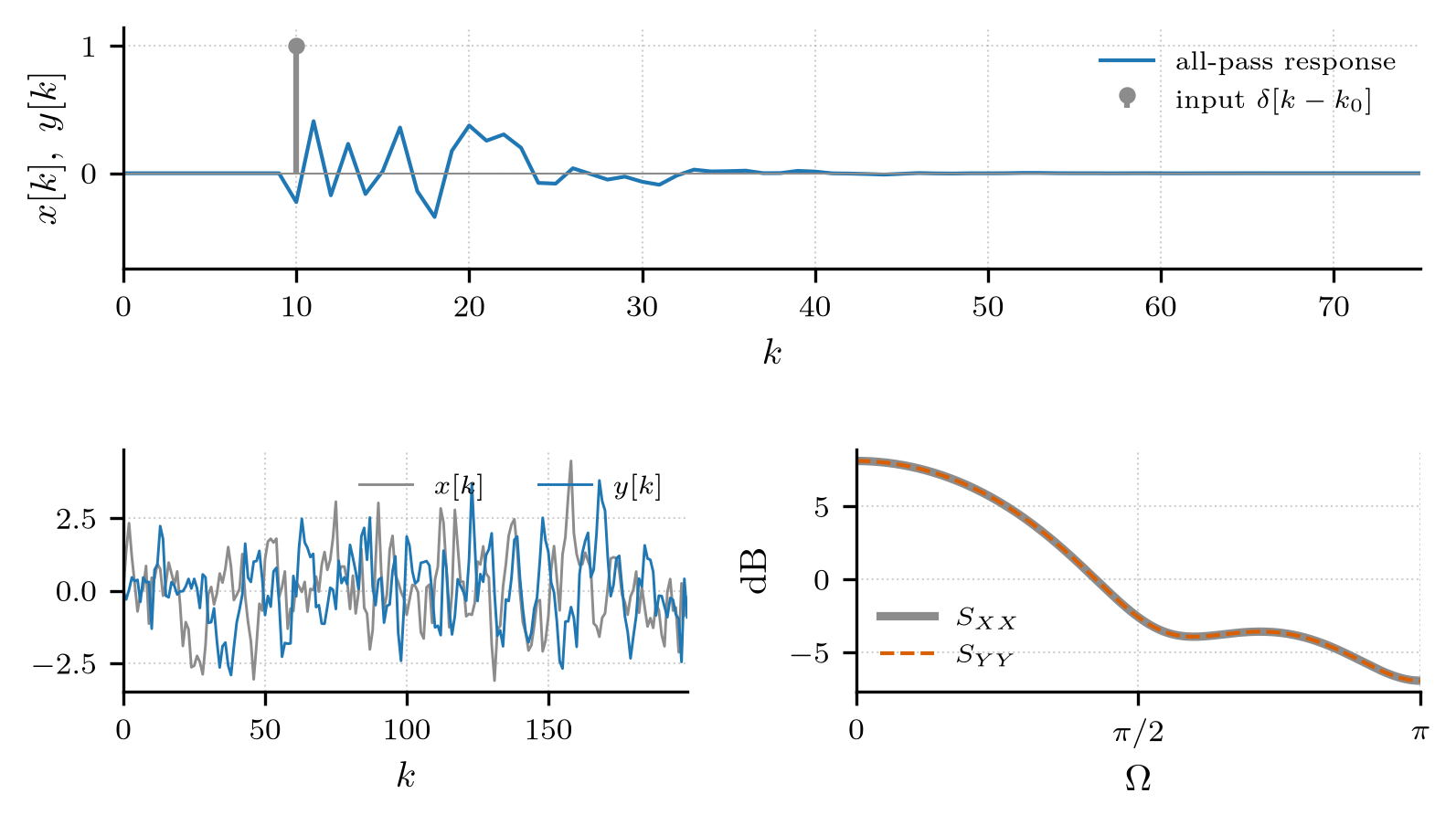
Any \(G\) with \(\abs{G}^2S_{XX}=1\) whitens, so whitening a process is not unique either. Causality picks one whitener, exactly as it picked Cholesky.

Back to a finite window

The correlation is a convolution

For a WSS process the correlation acts on a sequence as \((\mathcal Rx)[k]=\sum_lR_{XX}[k-l]\,x[l]\), a convolution. Feed in \(e^{j\Omega l}\): \[\sum_\lambda R_{XX}[\lambda]\,e^{j\Omega(k-\lambda)}=S_{XX}(e^{j\Omega})\;e^{j\Omega k} .\]

Fourier is the KLT of every stationary process The complex exponentials are the eigenfunctions, and the PSD is the eigenvalue spectrum: the eigendecomposition done once, for every stationary process at once. Exact for the whole process; a finite window’s Toeplitz matrix is diagonalized by the DFT only approximately (exactly if circulant).

Fourier decorrelates

Figure 10: An AR(1) process with pole 0.85: adjacent time samples (left) and adjacent DFT coefficients of 64-sample blocks (right).

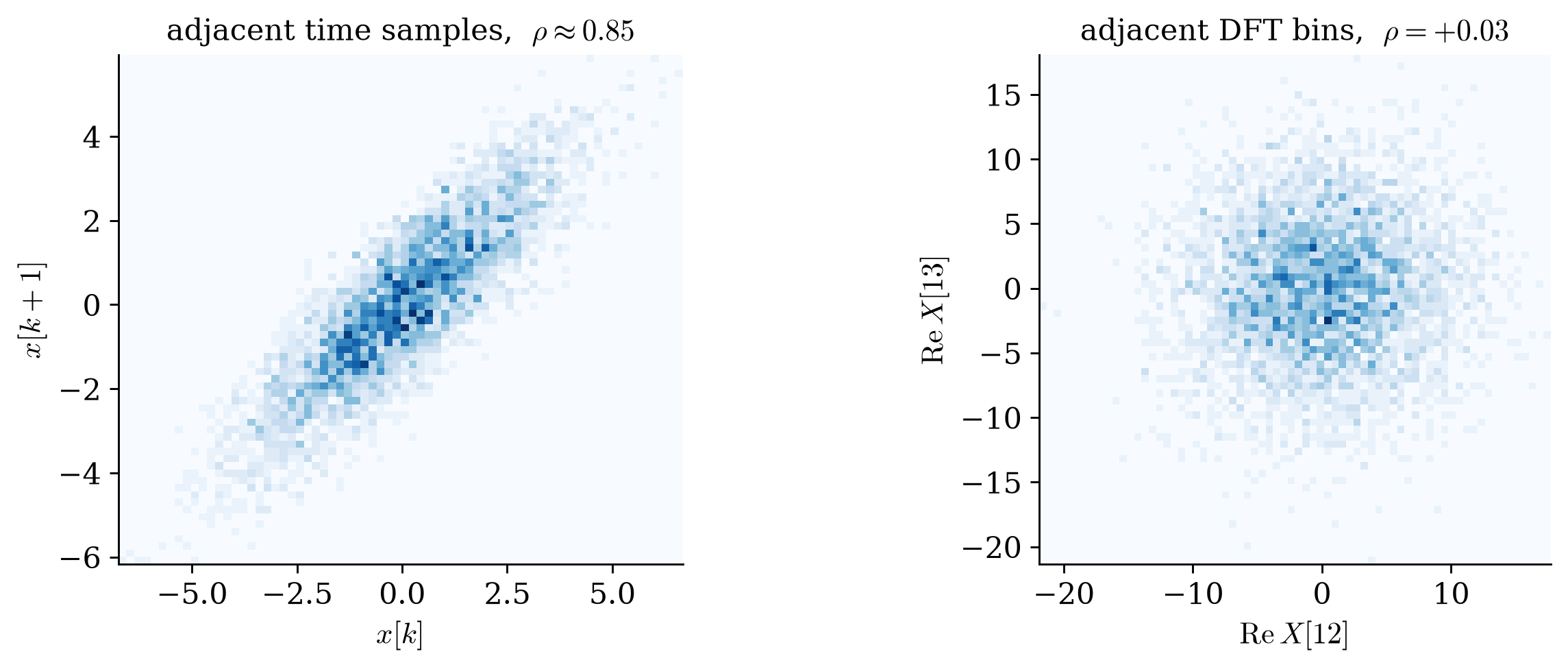
The transform decorrelated the process without ever being told its covariance.

A finite window is Toeplitz

The correlation as a function of the lag, and the same numbers as a matrix constant along every diagonal; a record of \(N\) samples sees only the solid window.

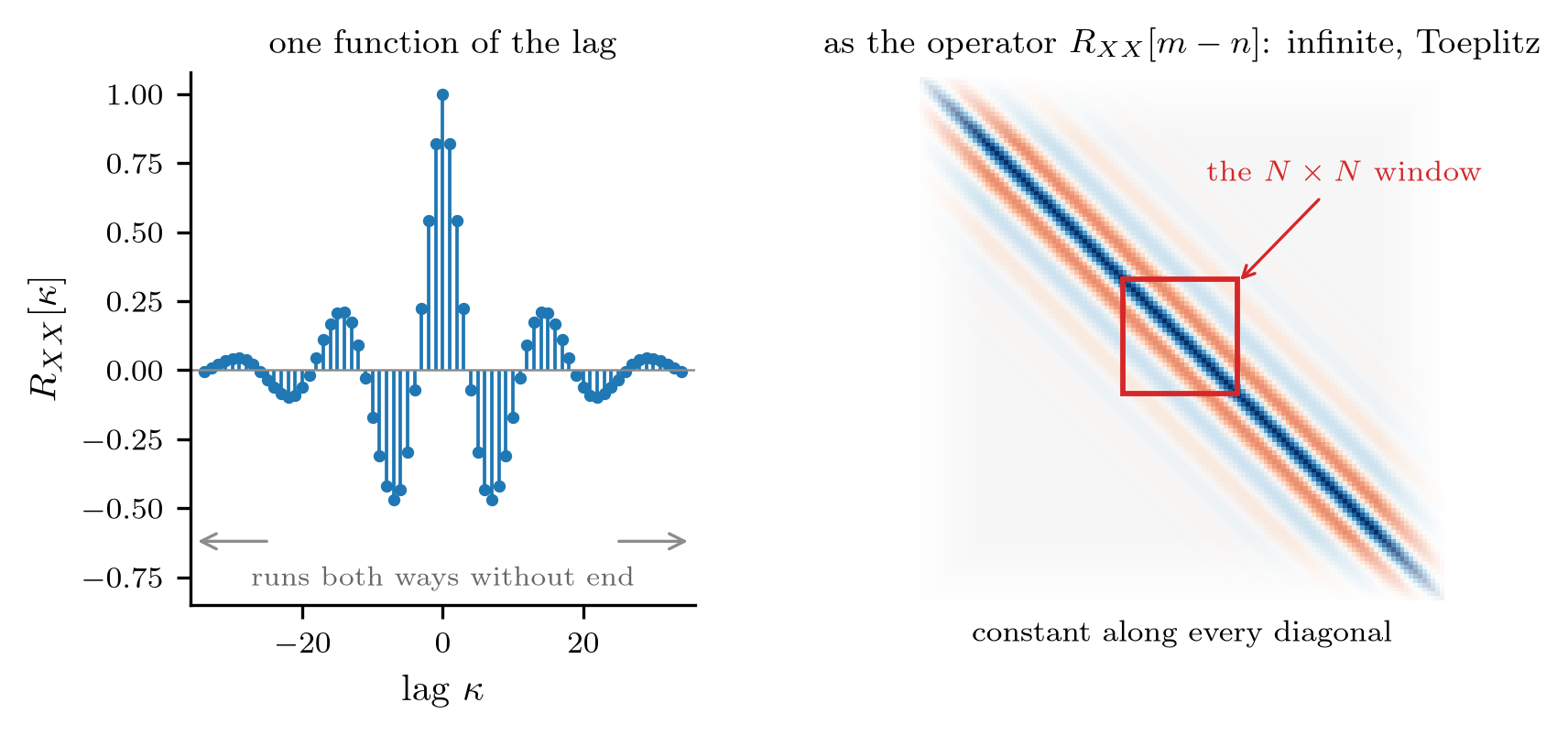
Cutting out \(N\) samples truncates the convolution. Complex exponentials are no longer exactly the eigenvectors, and what survives is a bound.

Toeplitz and circulant

A Toeplitz window and the circulant built by wrapping it: they differ only in the corners. The circulant’s eigenvalues are exactly the PSD samples and its eigenvectors the DFT columns; the Toeplitz eigenvectors are the same sinusoids, tapered at the ends.

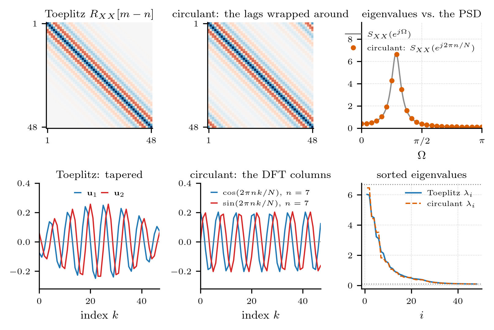
Exact on the circle, approximate on the line, and the corners matter less and less as the window grows.

The eigenvalues cannot leave the spectrum

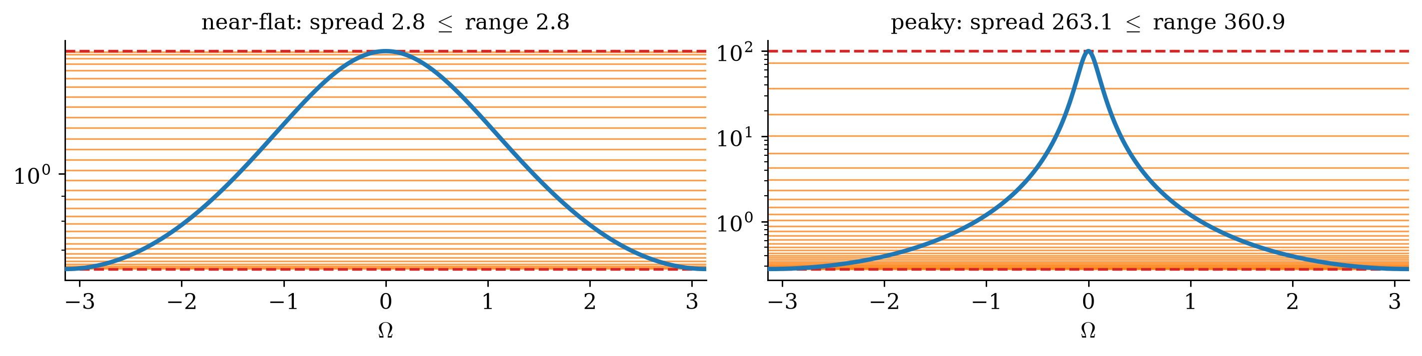
Eigenvalue spread and the PSD The eigenvalues of the \(N\times N\) Toeplitz correlation matrix lie between the extrema of the PSD, \(\min S_{XX}\le\lambda_i\le\max S_{XX}\), so \(\lambda_{\max}/\lambda_{\min}\le\max S_{XX}/\min S_{XX}\).

Why. For a unit eigenvector \(\mathbf q\) with spectrum \(Q\), \(\lambda=\mathbf q\herm\mathbf R\mathbf q=\frac{1}{2\pi}\int S_{XX}\abs{Q}^2\dd\Omega\): an average of the spectrum, which cannot leave its range. An eigenvalue is the process’s power seen through the filter \(\mathbf q\).

Figure 11: Two spectra, with the eigenvalues of their N = 32 Toeplitz correlation matrices drawn as horizontal levels.

How fast the two pictures meet

Figure 12: Sorted Toeplitz eigenvalues against the sorted PSD samples of the matching circulant, at three window lengths, for an AR(1) process with pole 0.9.

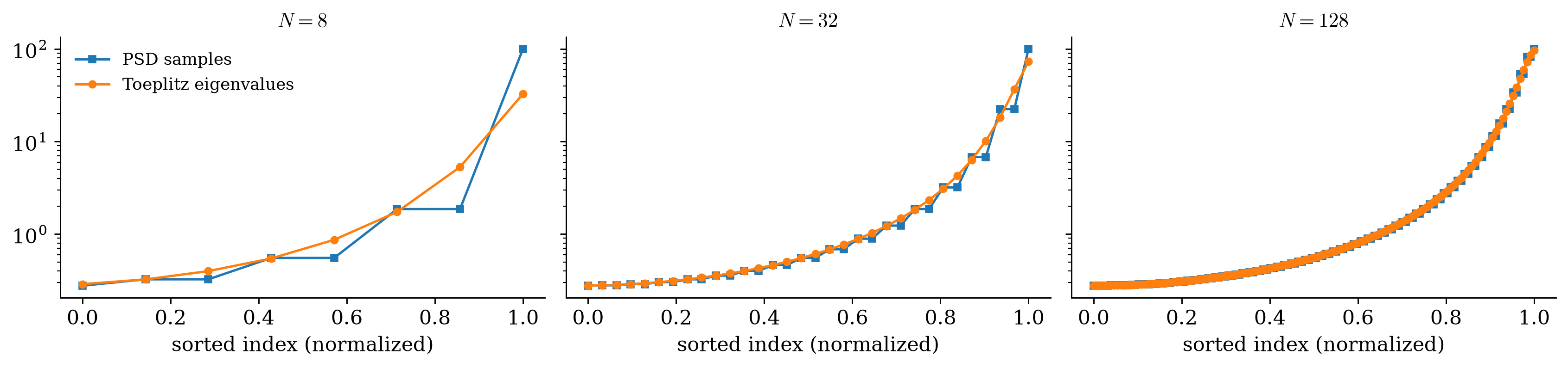
The eigenvalues of a finite window approach the spectrum as the window grows (Szegő), slowest where the spectrum is steepest. A short window cannot build a filter selective enough to sit on a sharp peak.

Truncating the spectral representation

A sinusoid in noise: its eigenvalue spectrum (the PSD) with two retained bins, and the rank-two reconstruction against the noisy realization and the true tone.

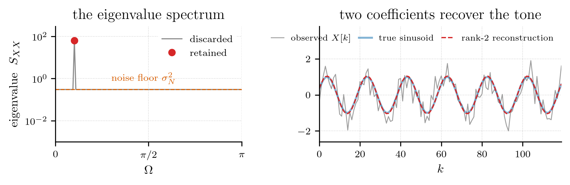
The KLT of the random-vector week, for a process: keep the strong eigen-directions, drop the noise floor. Two frequency coefficients recover the tone up to the noise that fell inside those two bins.

Why JPEG uses the DCT

\(8\times8\) image blocks: the KLT basis computed from the data, the DCT basis, and how much energy each packs into its first coefficients.

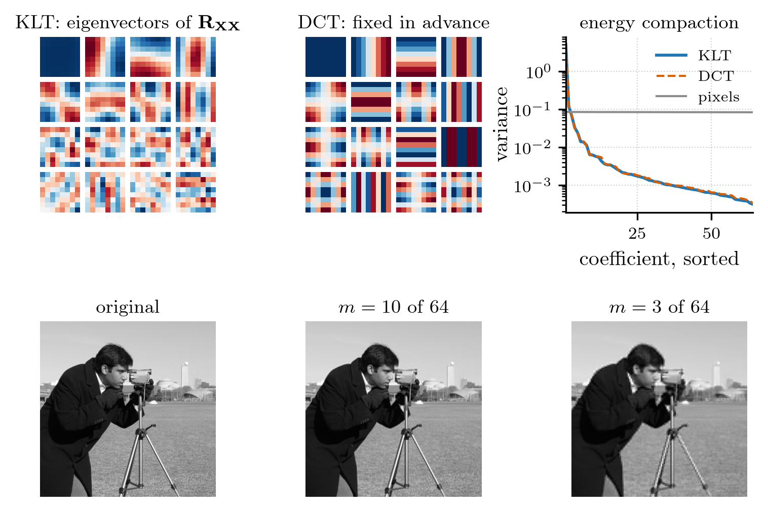
Image blocks are nearly stationary, so their KLT is nearly a cosine transform: the DCT gets almost all of the energy compaction without computing or transmitting any eigenvectors.

Recap

This week

1. A stationary process is a random vector whose correlation depends only on the lag. White noise is the identity covariance; one realization suffices when correlations die out (ergodicity), and stationarity does not guarantee it.

2. The PSD is the Fourier transform of the autocorrelation, and a filter multiplies it by \(\abs{H}^2\). Every regular process is white noise through a causal, minimum-phase filter, and the inverse of that filter whitens.

3. The Fourier basis is the KLT of a stationary process: the eigenvectors are known in advance, the eigenvalues are the spectrum (approximately, for a finite window), and their spread is the spectrum’s dynamic range.