Why Noise Is Gaussian

One random variable, then many

A microphone with nothing to record

\[ % Number sets \newcommand{\Nat}{\mathbb{N}} \newcommand{\Integer}{\mathbb{Z}} \newcommand{\Real}{\mathbb{R}} \newcommand{\Complex}{\mathbb{C}} % Operators \newcommand{\SNR}{\operatorname{SNR}} \newcommand{\tr}{\operatorname{tr}} \newcommand{\re}{\operatorname{Re}} \newcommand{\im}{\operatorname{Im}} \newcommand{\sign}{\operatorname{sign}} \newcommand{\rect}{\operatorname{rect}} \newcommand{\sinc}{\operatorname{si}} \newcommand{\erf}{\operatorname{erf}} \newcommand{\erfc}{\operatorname{erfc}} \newcommand{\kurt}{\operatorname{kurt}} \newcommand{\diag}{\operatorname{diag}} \newcommand{\MSE}{\operatorname{MSE}} \newcommand{\argmin}{\operatorname*{argmin}} \newcommand{\argmax}{\operatorname*{argmax}} \newcommand{\bias}{\operatorname{bias}} \newcommand{\Bin}{\operatorname{Bin}} % Delimiters \newcommand{\paren}[1]{\left(#1\right)} \newcommand{\bracket}[1]{\left[#1\right]} \newcommand{\set}[1]{\left\{#1\right\}} \newcommand{\abs}[1]{\left\lvert #1 \right\rvert} \newcommand{\norm}[1]{\left\lVert #1 \right\rVert} \newcommand{\ip}[1]{\left\langle #1 \right\rangle} % Notation \newcommand{\dd}{\,\mathrm{d}} \newcommand{\tran}{^{\top}} \newcommand{\conv}{\ast} \newcommand{\conj}{^{*}} \newcommand{\herm}{^{\mathsf{H}}} \newcommand{\opt}{^{\star}} % Expectation and variance % \newcommand{\E}[1]{\mathbb{E}\!\left[#1\right]} \newcommand{\E}[2][]{\mathbb{E}_{#1}\!\left[#2\right]} \newcommand{\Var}[1]{\mathbb{V}\!\left[#1\right]} % Distributions \newcommand{\Gauss}{\mathcal{N}} \newcommand{\Uniform}{\mathcal{U}} \newcommand{\FT}{\mathcal{F}} % Probability \newcommand{\Prob}[1]{\mathbb{P}\!\left(#1\right)} % Misc \newcommand{\bsy}[1]{\boldsymbol{#1}} \newcommand{\calR}{\mathcal{R}} \newcommand{\calC}{\mathcal{C}} \]

Listen to silence

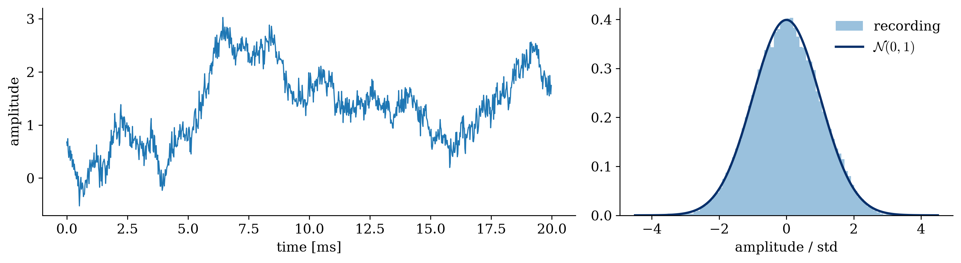
A studio microphone in a quiet room, recording nothing. What comes out is its self-noise.

Figure 1: Left: 20 ms of the recording. Right: the histogram of all 2 s of it, normalized to unit variance, against the Gaussian density.

Nobody told the microphone to be Gaussian. Why is it? This week answers that question, and the answer is why nearly every model in this course starts from a Gaussian.

The excess kurtosis of this recording is about −0.05; a Gaussian has 0. The whole week builds the two ideas needed to explain it: what a random variable is, and what happens when many independent ones are added.

The plan for the week

One number. A measurement is a random variable: a map from outcomes to numbers, described by a density and summarized by two moments.

Many numbers. Repeat the measurement, or add up many independent causes. Means add, variances add, and the shape of the sum forgets almost everything else.

In the notes Definition of a Random Variable · Distribution and Density · A Catalog of Distributions · Expectation and Moments · The Independent Sample · Sums of Independent Random Variables · Central Limit Theorem

One number

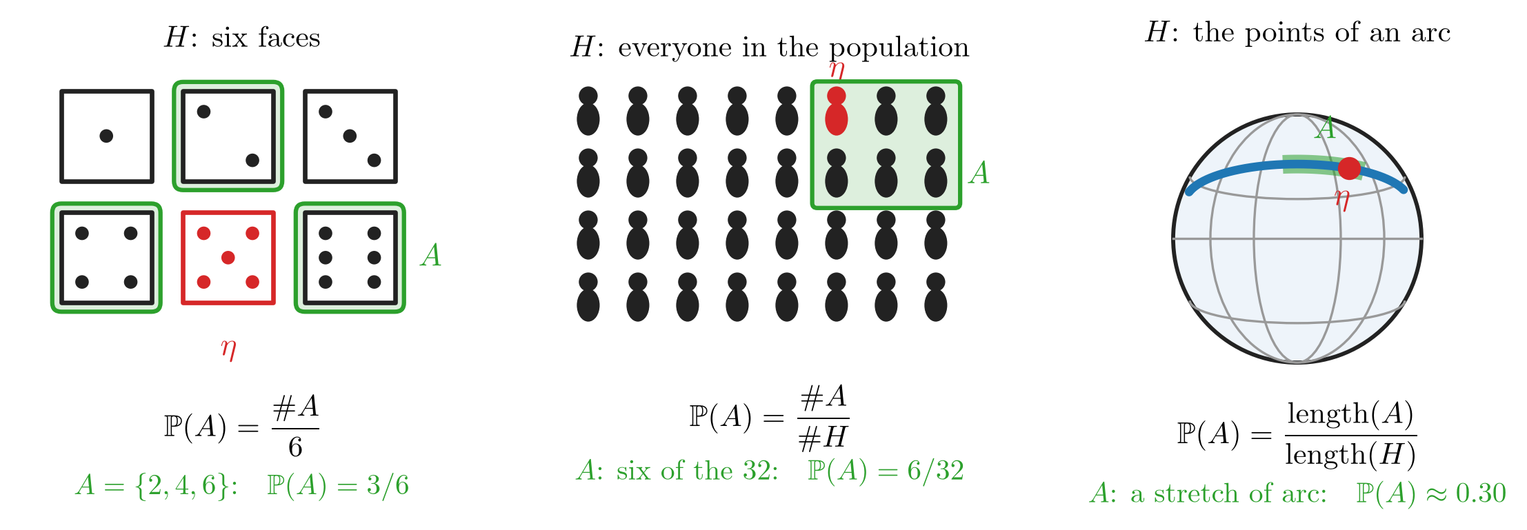
The probability space, in one slide

\((H,\mathcal{A},\Prob{\cdot})\)

• the sample space \(H\): every outcome \(\eta\) the experiment can produce, exactly one of which occurs;
• the events \(\mathcal{A}\): the subsets \(A\subseteq H\) we may ask about;
• the probability: one number per event, with \[\Prob{A}\ge 0,\qquad \Prob{H}=1,\qquad \Prob{A\cup B}=\Prob{A}+\Prob{B}\ \text{ for disjoint } A,B.\]

The probability space, in one slide

One outcome \(\eta\) in red, one event \(A\) in green: probability counts faces, counts people, then measures length.

Notice what is not in the triple: numbers. Probability lives on sets of outcomes.

A random variable is a map

An experiment produces an outcome \(\eta\). Signal processing needs the number read from it.

Random variable \[X:H\to\Real,\qquad x = X(\eta).\] The map is deterministic. The randomness is in which outcome occurs.

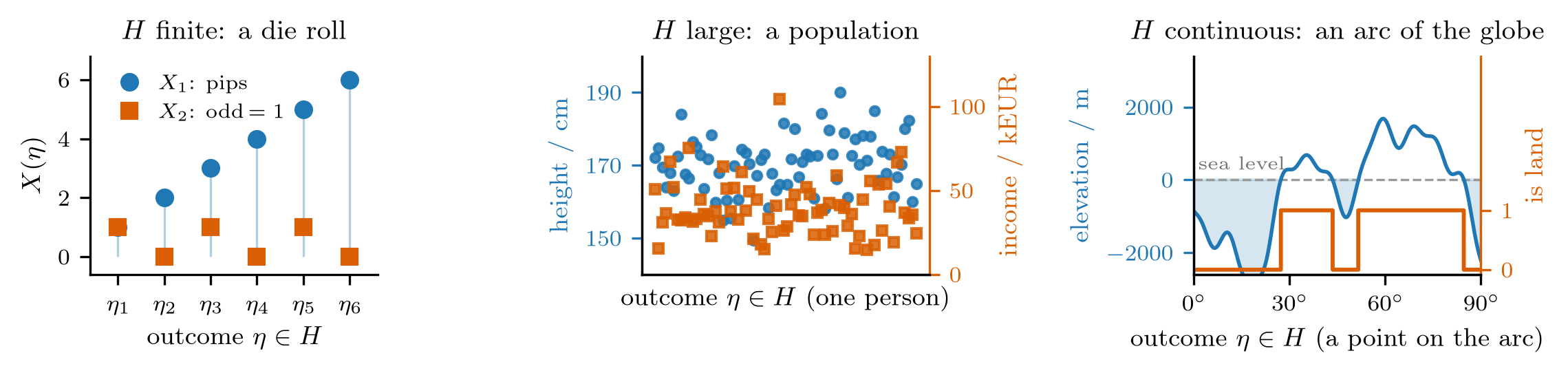
Two maps on each of three sample spaces.

The law of a random variable

Everything about \(X\) is in the probability of the threshold events \(\set{X\le x}\):

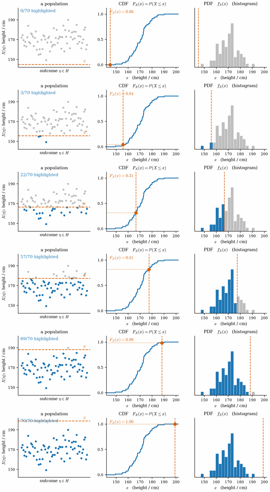
Cumulative distribution function (CDF) and probability density function (PDF) \[F_X(x)=\Prob{X\le x},\qquad f_X(x)=\frac{\dd F_X(x)}{\dd x},\qquad \Prob{x<X\le x+\Delta}\approx f_X(x)\,\Delta .\]

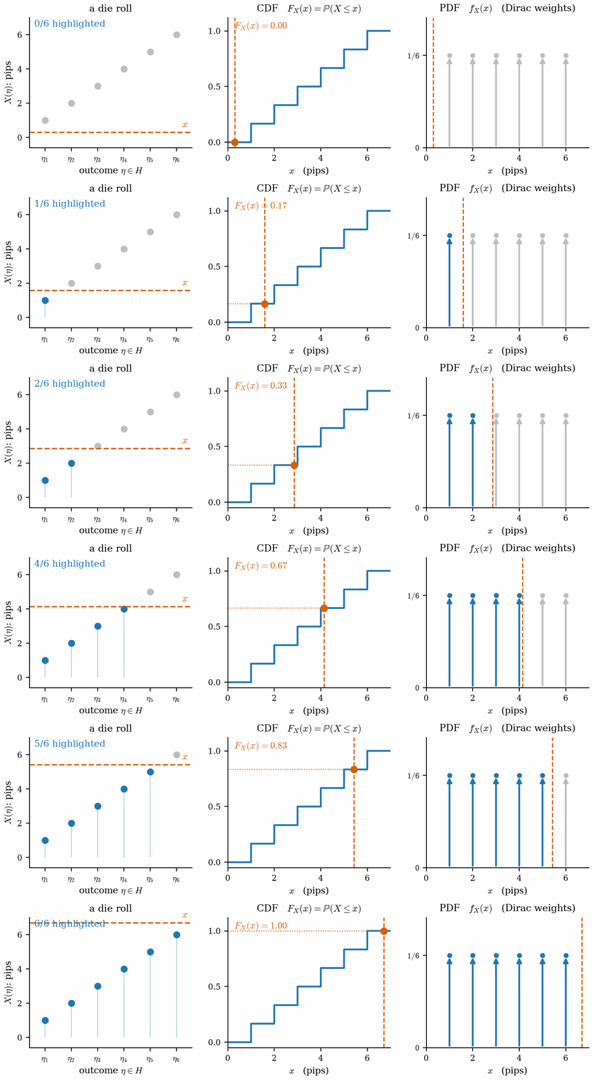
Sweeping the level \(x\) over the die: the outcomes below it, the CDF, the density.

Sweeping the level: a population

The same sweep over 70 people, with height as the map.

Strictly a staircase, 70 outcomes and 70 steps, but at this resolution the steps are invisible and the law is read as a smooth CDF with a density beneath it. That is the whole justification for modeling a population as continuous.

Sweeping the level: an arc of terrain

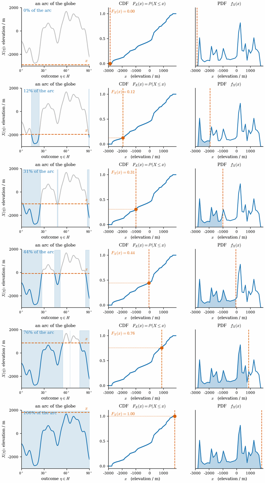
Elevation along an arc; the highlighted bands are the stretches below \(x\).

No steps and no atoms: the density is genuinely a rate. It is high where the terrain is flat, because the profile lingers there and more of the arc falls in that band of elevations.

Density is probability per unit length

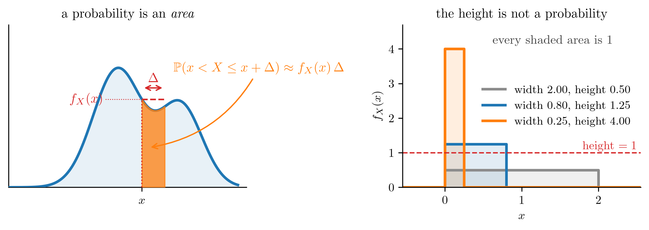
Left: a probability is the area of a strip. Right: three uniform densities of unit area.

Only areas under a density are probabilities. Its height can exceed one, and any single value of a continuous variable has probability zero.

Laws that recur by name

Each law is the signature of a mechanism

Law	Density or weights	Where it comes from
Bernoulli \((p)\)	\(\Prob{X=1}=p\)	one event: occurred or not
Binomial \(\Bin(N,p)\)	\(\binom Nk p^k(1-p)^{N-k}\)	successes in \(N\) independent trials
Poisson \((a)\)	\(e^{-a}a^k/k!\)	many rare, independent chances
Uniform \([x_{\min},x_{\max}]\)	flat	bounded, no value preferred: a quantization error, a phase
Gaussian \(\Gauss(m,\sigma^2)\)	\(\frac{1}{\sqrt{2\pi}\sigma}e^{-(x-m)^2/2\sigma^2}\)	the aggregate of many small effects
Laplacian	\(\frac{1}{2b}e^{-\abs{x-a}/b}\)	a sharp peak with heavy tails: clicks, outliers
Cauchy	\(\frac{1}{\pi(1+x^2)}\)	a ratio of Gaussians; the cautionary tale

The right-hand column is the point; by the end of the week the Gaussian’s entry is a theorem.

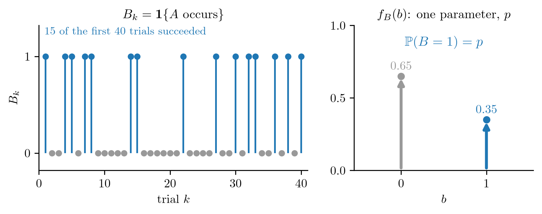
Coin Flip: Bernoulli

An iid Bernoulli sequence and its two-weight law.

Counting: Binomial

Repeat the coin flip \(N\) times and count the heads \(K\); \(\binom Nk\) sequences have \(k\) heads: \[\Prob{K=k}=\binom Nk p^k(1-p)^{N-k},\qquad k=0,\dots,N .\]

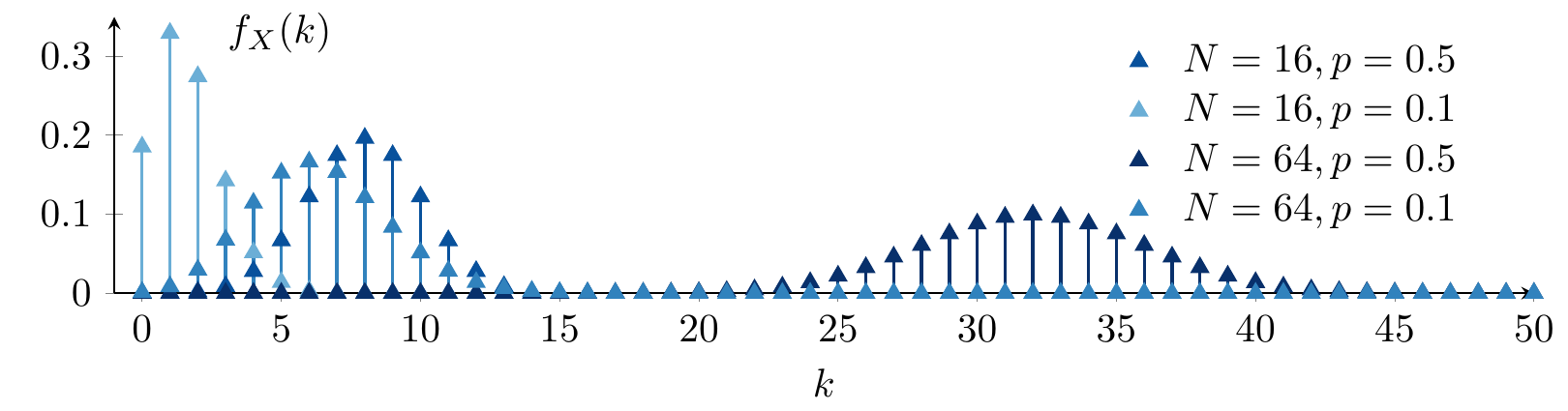
The binomial law for two trial counts and two event probabilities.

A binomial count is a sum of \(N\) Bernoulli indicators. It peaks near \(Np\) and, as \(N\) grows, it already looks Gaussian: a first hint of the week’s answer.

The uniform: bounded, nothing preferred

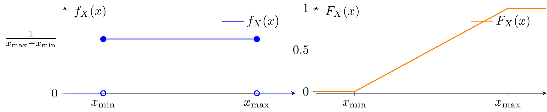
Density and CDF of \(\Uniform[x_{\min},x_{\max}]\).

A flat density, a straight-ramp CDF. The law of a quantization error, of a phase known only up to \(2\pi\), and of a position along the arc.

The Gaussian: two parameters you can read off

\[f_X(x)=\frac{1}{\sqrt{2\pi}\,\sigma}\,e^{-(x-m)^2/2\sigma^2}\]

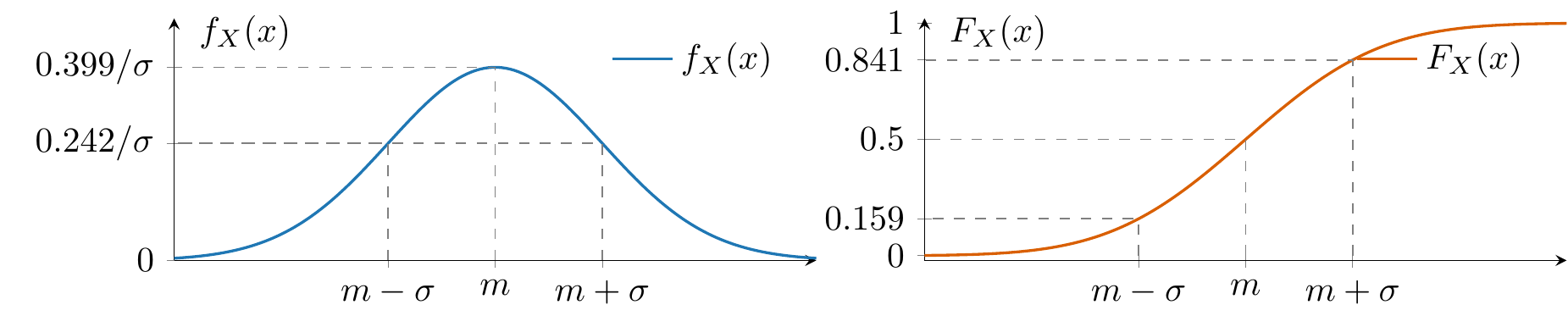
Density and CDF of \(\Gauss(m,\sigma^2)\).

\(m\) is the peak and the median. \(\sigma\) is the distance from the peak to the inflection point. About two thirds of the mass lies within one \(\sigma\).

Expectation

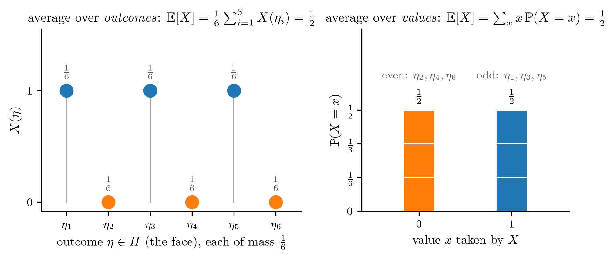
Expectation is an ensemble average

Expectation The average of the map over all equally likely outcomes: \[\E{X}=\frac{1}{\abs{H}}\int_H X(\eta)\dd\eta\qquad\Bigl(\text{discrete: } \tfrac{1}{\abs{H}}\textstyle\sum_{\eta\in H} X(\eta)\Bigr).\] The same normalization as \(\Prob{A}=\abs{A}/\abs{H}\): probability is a fraction of outcomes, expectation an average over them.

Expectation from the density Group the outcomes by the value they produce: \[\E{X}=\int_{-\infty}^{\infty}x\,f_X(x)\dd x\qquad\Bigl(\text{discrete: } \textstyle\sum_i x_i\,\Prob{x_i}\Bigr).\]

Expectation is an ensemble average

A fair die, \(X=1\) on an odd face: averaged over outcomes (left) and over values (right).

Expectation is an ensemble average

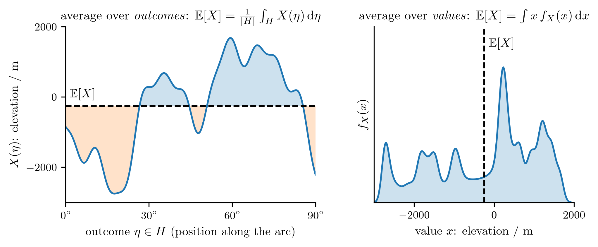
Elevation along the arc, averaged over outcomes (left) and over values (right). On the sample space the mean is a level, a horizontal line; on the value axis it is the balance point of \(f_X\), a vertical line.

The right-hand axis is the only one available in practice: we model or measure the density, never the sample space. Nothing is lost, because the grouping is exactly \(f_X\).

Any function averages against the same density

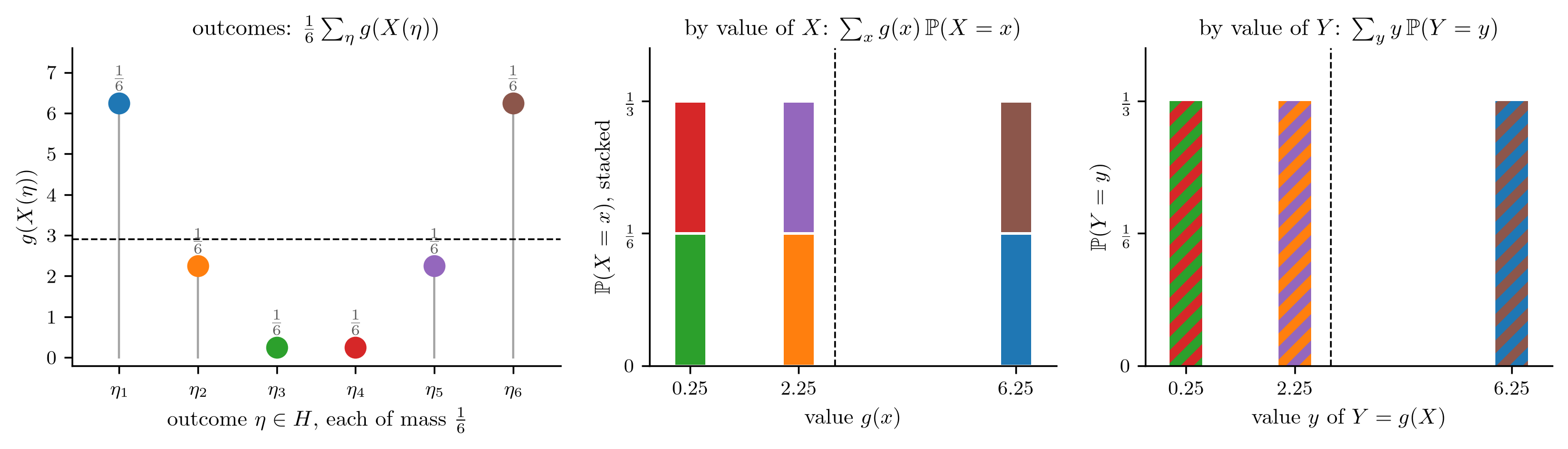
\(g(X)\) is again a map on \(H\), \(\eta\mapsto g(X(\eta))\), so the definition applies. Group its outcomes by the value of \(X\), not by the value of \(g(X)\): \[\E{g(X)}=\frac{1}{\abs{H}}\sum_{\eta\in H} g\bigl(X(\eta)\bigr) =\sum_x g(x)\,\frac{\abs{\{X=x\}}}{\abs{H}}=\sum_x g(x)\,\Prob{X=x}.\]

Law of the unconscious statistician For \(Y=g(X)\) (the law of \(Y\) is never needed): \[\E{g(X)}=\int_{-\infty}^{\infty}g(x)\,f_X(x)\dd x\qquad\Bigl(\text{discrete: } \textstyle\sum_i g(x_i)\,\Prob{x_i}\Bigr).\]

Any function averages against the same density

A fair die and \(g(x)=(x-\tfrac72)^2\), so \(\E{g(X)}=\tfrac{35}{12}\). Each outcome in its own colour (left), stacked by the value of \(X\) (middle), and blended into the law of \(Y=g(X)\) (right). The middle sum already has the answer; the law of \(Y\) only forgets which outcomes merged.

Linearity is the workhorse

For constants \(a,b\) and functions \(g_k\) of the same \(X\): \[\E{a\,g(X)+b}=a\,\E{g(X)}+b,\qquad \E{\textstyle\sum_k a_k\,g_k(X)}=\sum_k a_k\,\E{g_k(X)}.\] Immediate from linearity of the integral \(\int g(x)\,f_X(x)\dd x\).

A die \(\E{X}=\tfrac{7}{2}\) and \(\E{X^2}=\tfrac{91}{6}\). Without ever finding the law of \((X-1)^2\): \[\E{(X-1)^2}=\E{X^2}-2\,\E{X}+1=\tfrac{91}{6}-7+1=\tfrac{55}{6}.\]

Almost every derivation in this course is this one line used again: expectation passes through sums, and through filters, transforms and matrices, which are sums.

Two numbers carry forward

Mean and variance \[m_X=\E{X},\qquad \sigma_X^2=\Var{X}=\E{(X-m_X)^2}.\]

Expand the square and use linearity: \[\sigma_X^2=\E{X^2}-2m_X\E{X}+m_X^2=\E{X^2}-m_X^2 .\]

For an affine map \(Y=aX+b\): \[\begin{aligned} m_Y&=a\,m_X+b,\\ \sigma_Y&=\lvert a\rvert\,\sigma_X .\end{aligned}\] Scaled by \(a\), untouched by the shift.

\(m_X\) locates, \(\sigma_X^2\) measures the mean-square spread around it. Setting \(m_X=0\) changes nothing about the spread, which is why the course mostly works with zero-mean variables.

What each moment listens to

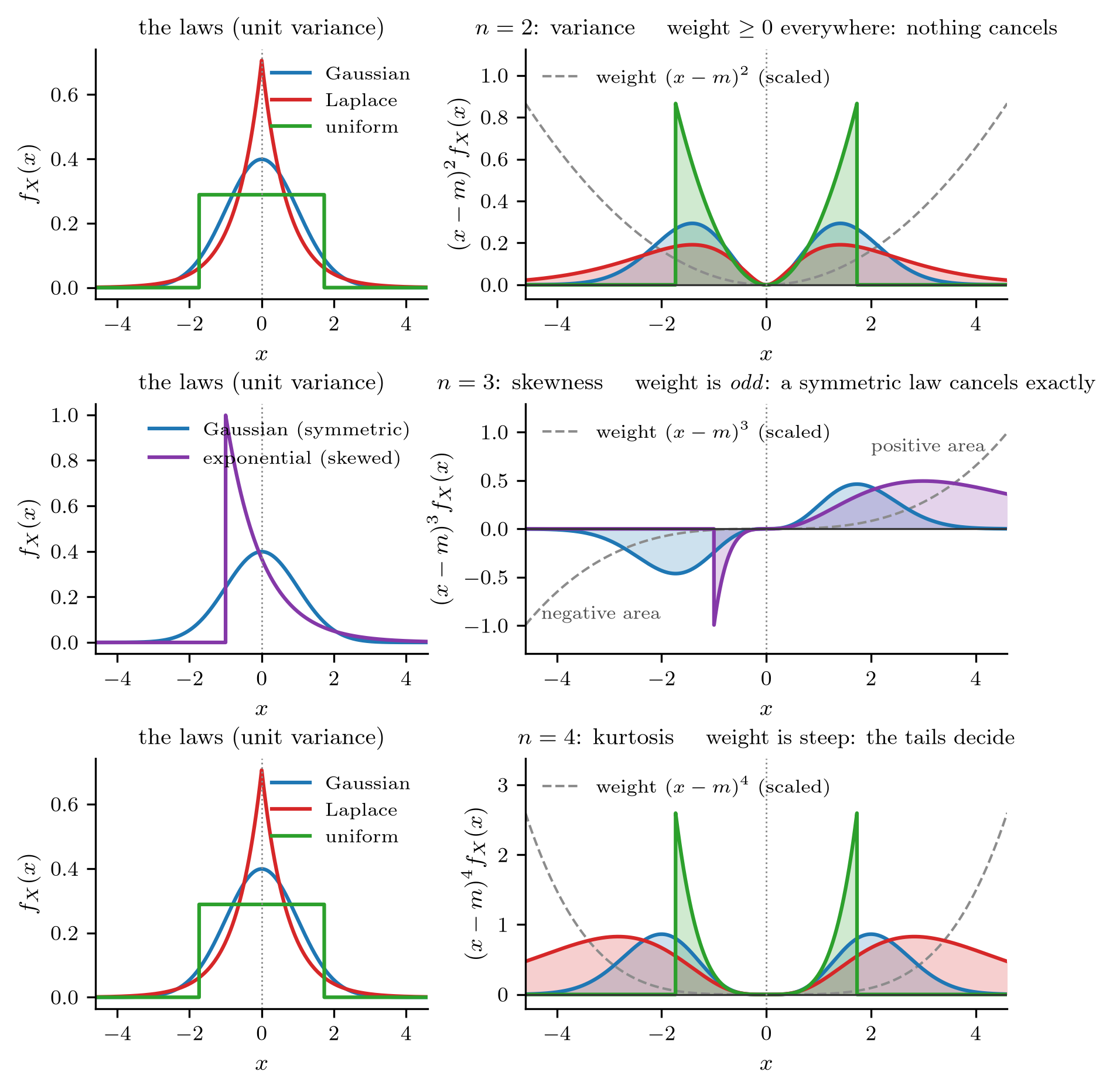
Laws of unit variance, and the integrand \((x-m_X)^nf_X(x)\) whose area is the \(n\)-th central moment, for \(n=2,3,4\).

\[\mu^{(n)}_X=\E{(X-m_X)^n}=\int_{-\infty}^{\infty}(x-m_X)^n\,f_X(x)\dd x\]

\(n=2\) reads the shoulders: the variance.

\(n=3\) (skewness) cancels for symmetric laws.

\(n=4\) (kurtosis) is decided by the tails, so laws of equal variance separate. The kurtosis is how the opening recording was judged Gaussian.

The named laws, moment by moment

Normalized: skewness \(\mu^{(3)}_X/\sigma_X^3\), excess kurtosis \(\mu^{(4)}_X/\sigma_X^4-3\).

Law	\(m_X\)	\(\sigma_X^2\)	skewness	excess kurtosis
Bernoulli \((p)\)	\(p\)	\(p(1-p)\)	\(\frac{1-2p}{\sqrt{p(1-p)}}\)	\(\frac{1-6p(1-p)}{p(1-p)}\)
Binomial \(\Bin(N,p)\)	\(Np\)	\(Np(1-p)\)	\(\frac{1-2p}{\sqrt{Np(1-p)}}\)	\(\frac{1-6p(1-p)}{Np(1-p)}\)
Poisson \((a)\)	\(a\)	\(a\)	\(\frac{1}{\sqrt a}\)	\(\frac1a\)
Uniform \([x_{\min},x_{\max}]\)	\(\frac{x_{\min}+x_{\max}}{2}\)	\(\frac{(x_{\max}-x_{\min})^2}{12}\)	\(0\)	\(-\frac65\)
Gaussian \(\Gauss(m,\sigma^2)\)	\(m\)	\(\sigma^2\)	\(0\)	\(0\)
Laplacian \((a,b)\)	\(a\)	\(2b^2\)	\(0\)	\(3\)
Cauchy	none	none	none	none

The excess kurtosis orders the tails: uniform \(<\) Gaussian \(<\) Laplacian. The binomial’s shape numbers shrink like \(1/\sqrt N\) and \(1/N\) towards the Gaussian’s zeros.

Standard deviation is the spread, not the shape

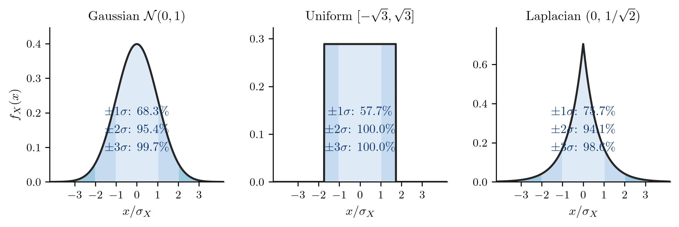
Three densities with the same \(\sigma_X\), and the mass within \(\pm1,2,3\,\sigma_X\).

Same spread, different shape: the uniform has nothing beyond \(1.73\,\sigma_X\), the Laplacian still \(1.4\%\) beyond \(3\,\sigma_X\). The 68–95–99.7 rule is a Gaussian statement. Two moments fix the scale, not how often something extreme happens.

The mean is the best constant guess

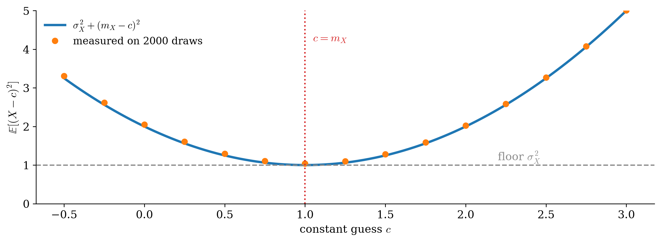
If you must summarize \(X\) by one constant \(c\), and you pay the squared error, split the error at the mean: \[\E{(X-c)^2}=\E{(X-m_X)^2}+2(m_X-c)\underbrace{\E{X-m_X}}_{=0}+(m_X-c)^2 =\underbrace{\sigma_X^2}_{\text{unavoidable}}+\underbrace{(m_X-c)^2}_{\text{your choice}} .\]

The best constant guess \(c=m_X\), and what is left over is the variance.

The first estimation problem of the course, already in its final shape: an error that splits into a part the estimator controls and a floor it cannot go below.

The best constant, drawn

Figure 2: Mean-square error of the constant guess c for an exponential variable (mean 1, variance 1): the formula and a Monte Carlo estimate from 2000 draws.

A parabola with its bottom at the mean and its floor at the variance, whatever the shape of the law: here a skewed exponential.

Many numbers

Repeating an experiment is one bigger experiment

Rolling a die twice is one experiment on the product space \(H\times H\), with two maps on it.

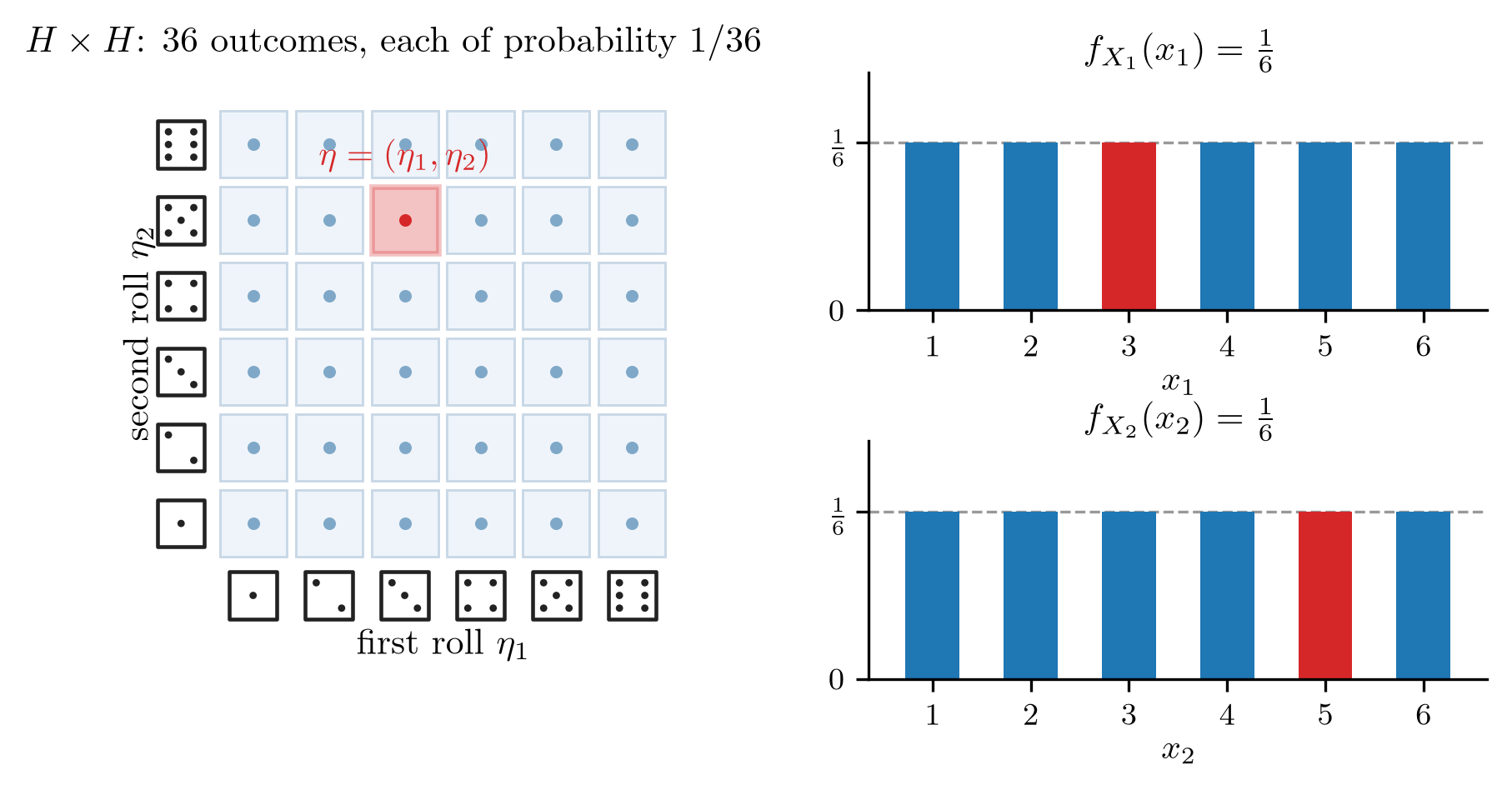
The 36 equally likely pairs, and each coordinate read on its own.

iid sample \(X_1,\dots,X_N\), each the same map on its own copy of the experiment: identically distributed, and independent.

Independence: the joint law is a product

For independent \(X_1,\dots,X_N\) the joint distribution and density factor, \[F_{\mathbf X}(\mathbf x)=\prod_{k=1}^{N}F_X(x_k),\qquad f_{\mathbf X}(\mathbf x)=\prod_{k=1}^{N}f_X(x_k).\]

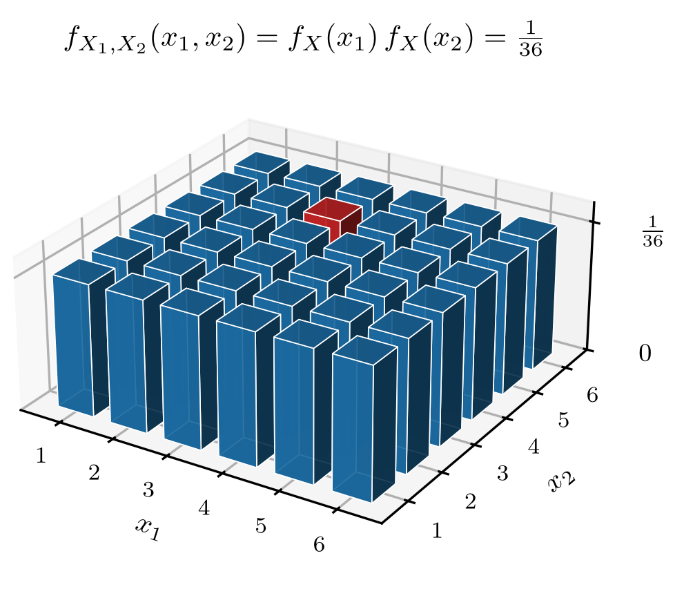
The pair of rolls: one flat weight \(\tfrac16\cdot\tfrac16\) per lattice point.

Counting is already estimation

The data are \(N\) Bernoulli trials; the only sensible estimate of \(p\) is the fraction: \(\widehat p_N=\frac1N\sum_k B_k\).

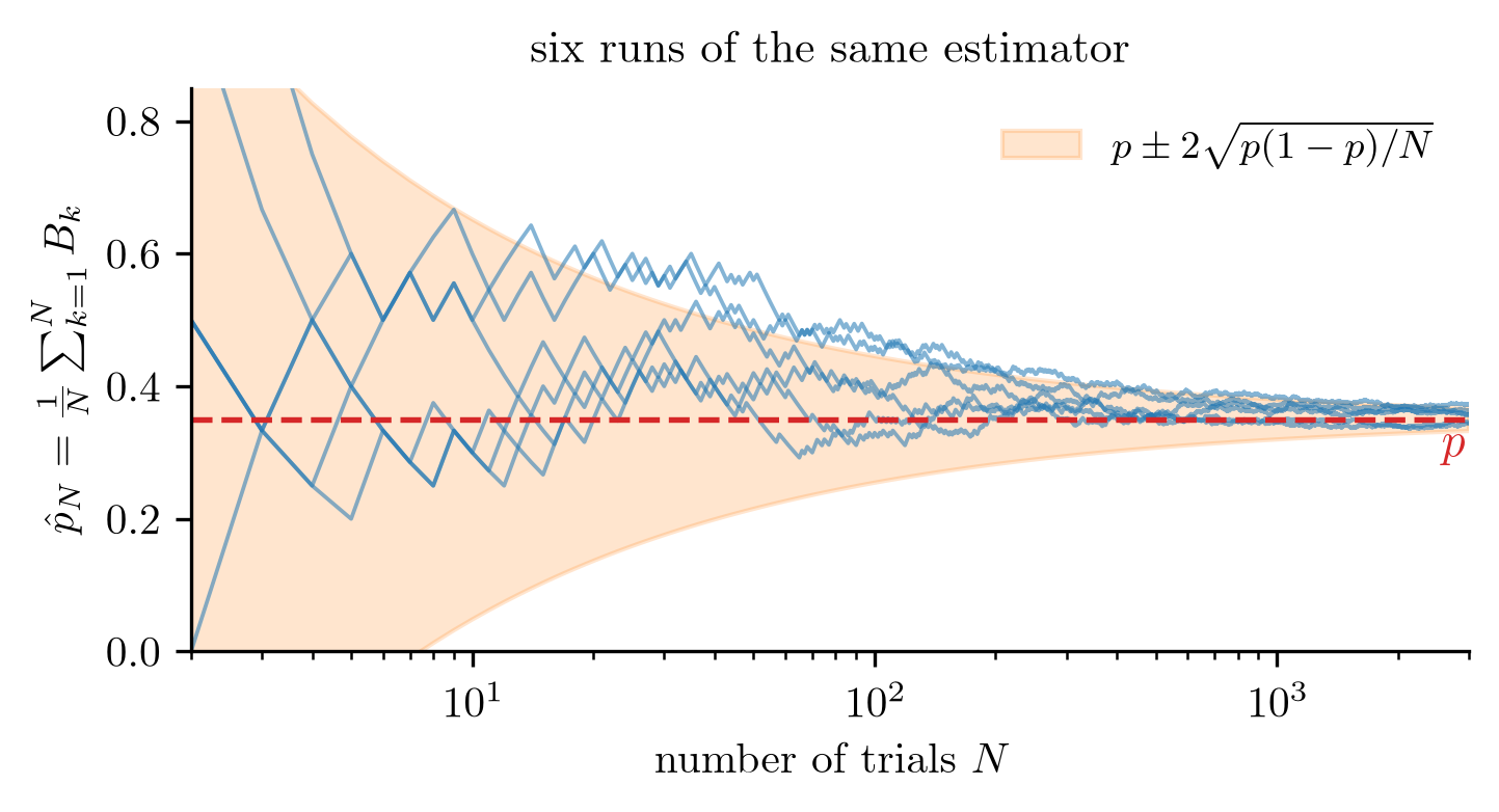
Six runs of the estimator against the true \(p\).

 

Every run gives a different number, so the estimate is itself a random variable. Its spread shrinks like \(1/\sqrt N\): the pattern estimate, then say how far off it can be.

Approximating \(\pi\) by counting

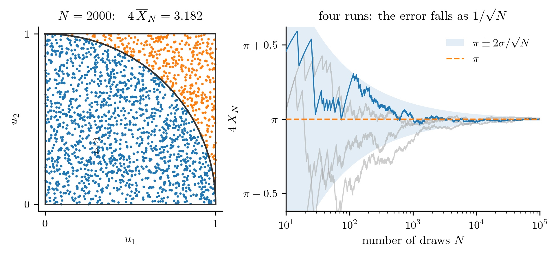
Points uniform in the unit square; the fraction inside the quarter disc estimates \(\pi/4\). Right: four independent runs, inside an envelope narrowing as \(1/\sqrt N\).

An area computed by counting. It does not care about dimension, which is why Monte Carlo survives where grids of quadrature points do not.

Independence splits expectations

Integrating against a product density separates the integral: \[\E{g(X)\,h(Y)}=\E{g(X)}\,\E{h(Y)}\qquad (X,Y \text{ independent}).\]

Now add. The mean of a sum is the sum of the means by linearity alone. For the variance, expand the square of the centered sum: \[\begin{aligned} \Var{X+Y}&=\E{\big((X-m_X)+(Y-m_Y)\big)^2}\\ &=\E{(X-m_X)^2}+\E{(Y-m_Y)^2}+2\,\E{(X-m_X)(Y-m_Y)}\\ &=\Var{X}+\Var{Y}+2\,\underbrace{\E{X-m_X}}_{=\;0}\,\E{Y-m_Y} . \end{aligned}\]

For independent variables, variances add. Sums always split under expectation; products split only under independence.

Why averaging helps, and how slowly

For the iid sample, \(N\) equal terms: \[\E{\overline X_N}=m_X,\qquad \Var{\overline X_N}=\frac{\sigma_X^2}{N},\qquad \overline X_N=\frac1N\sum_{k=1}^N X_k .\]

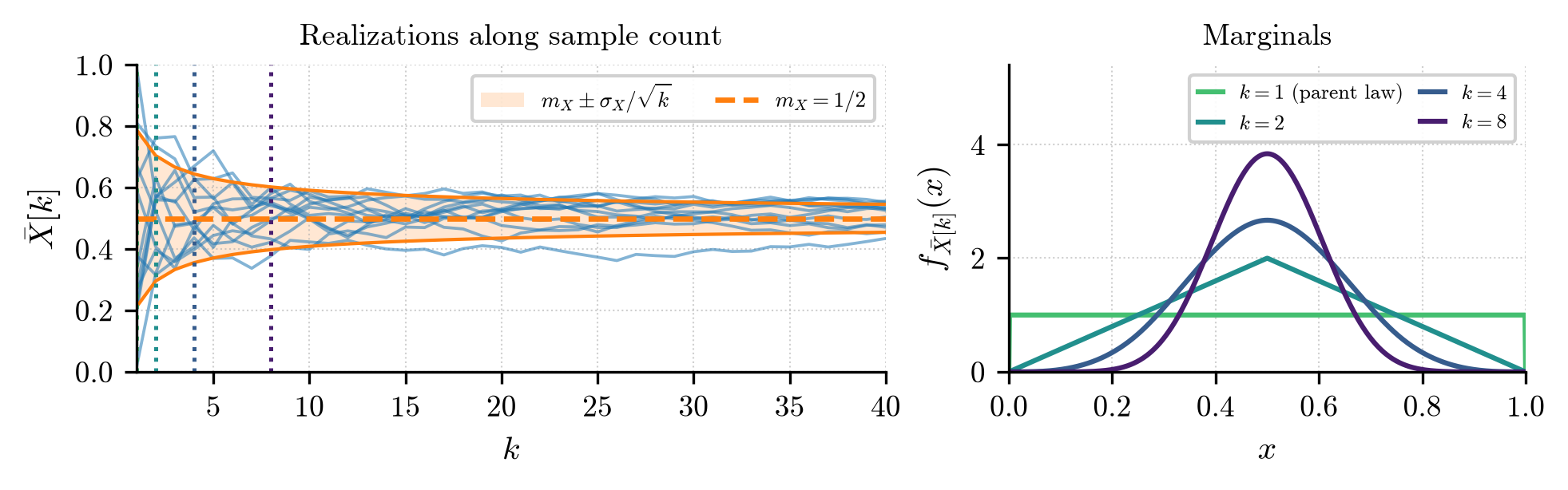
Left: running averages of uniform draws, inside \(m_X\pm\sigma_X/\sqrt k\). Right: the density of the average for \(k=1,2,4,8\).

Error falls as \(1/\sqrt N\): one more digit costs a hundred times the data. → Demo: the mean of \(N\) dice

The law of large numbers

The variance of the average goes to zero, and Chebyshev’s inequality turns that into a guarantee:

Law of large numbers \[\Prob{\abs{\overline X_N-m_X}\ge\epsilon}\le\frac{\sigma_X^2}{N\epsilon^2}\xrightarrow{N\to\infty}0 .\] The bound holds at every finite \(N\): the licence to replace an expectation by an average over data.

It says the average settles. It says nothing yet about the shape of the error around \(m_X\). That shape is the question the microphone asked.

Two dice: grouping the cells by their sum

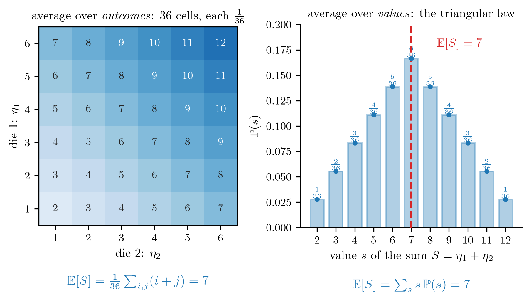
The sum of two dice. Left: the average over the 36 equally likely cells. Right: the same 36 terms collected by the value they produce.

Regrouping outcomes by value is the whole proof that the two formulas for \(\E{X}\) agree.

A sum smooths the density

The density of a sum of independent variables is the convolution of their densities, \(f_{X+Y}=f_X*f_Y\).

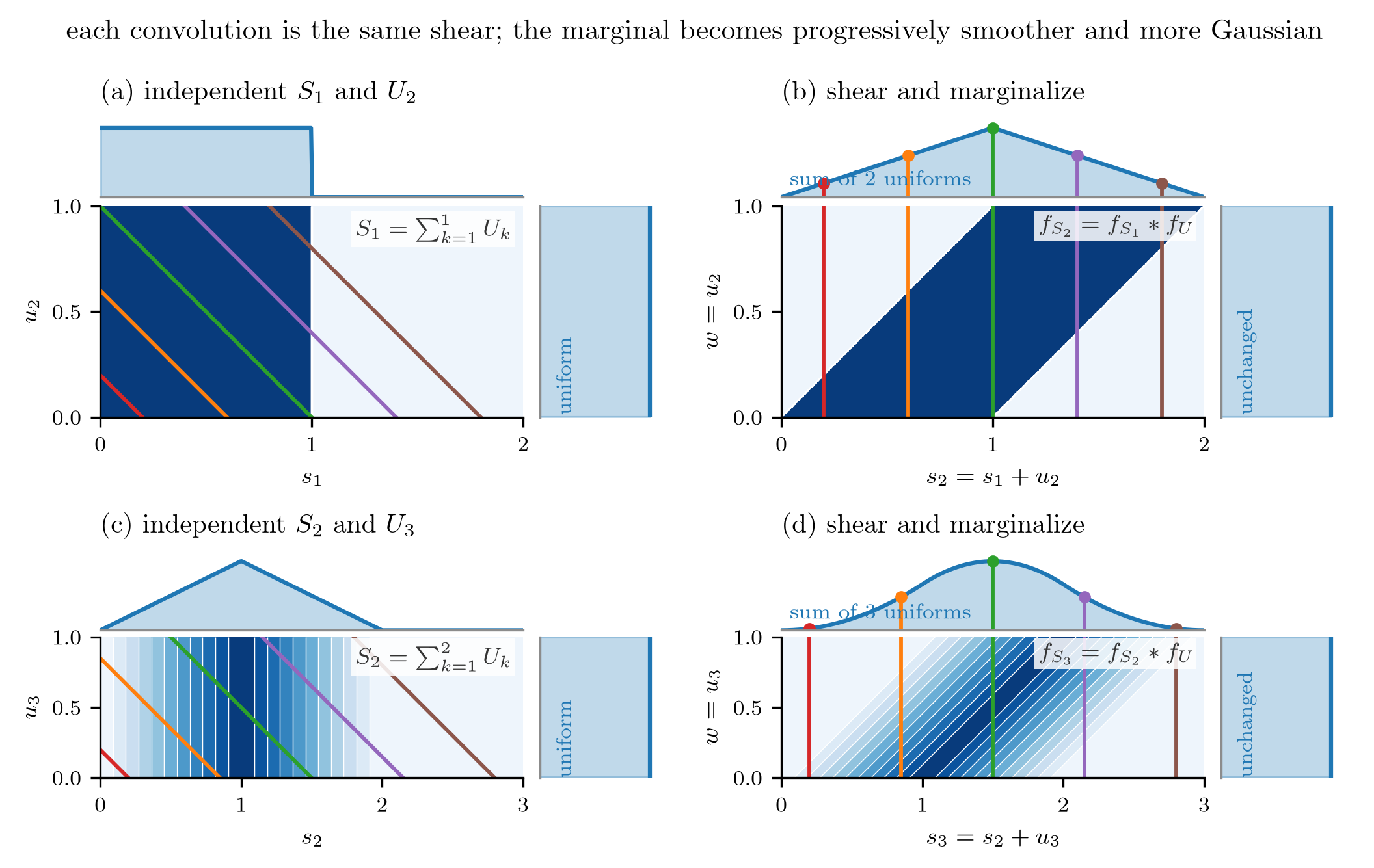
Each addition is the same smoothing step; after a few, the shape no longer remembers where it started.

Sums that stay in the family

 

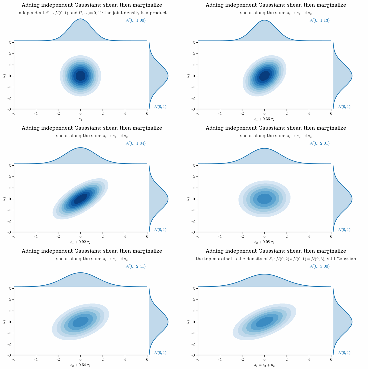
Some laws are closed under addition of independent copies:

• \(N\) Bernoulli\((p)\) indicators sum to \(\Bin(N,p)\): pooling two runs is one longer run.
• Independent Gaussians add their means and their variances, and stay Gaussian.

Among laws with finite variance, the Gaussian is the only one that keeps its shape when independent copies are added and rescaled: a fixed point. Everything else is drawn toward it.

The central limit theorem

Central limit theorem For iid \(X_k\) with finite mean \(m_X\) and variance \(\sigma_X^2\), \[\sqrt N\,\frac{\overline X_N-m_X}{\sigma_X}\;\xrightarrow{\ \mathcal D\ }\;\Gauss(0,1), \qquad\text{i.e.}\qquad \overline X_N\approx\Gauss\!\paren{m_X,\tfrac{\sigma_X^2}{N}} .\]

Everything about the parent law except its mean and variance washes out. What is left is the Gaussian: the one law fixed by two moments alone.

The proof in the notes runs through the cumulants: they add over independent summands, and after normalization every cumulant above the second is suppressed by a power of N. Say this in one sentence if asked.

Fast in the body, slow in the tails

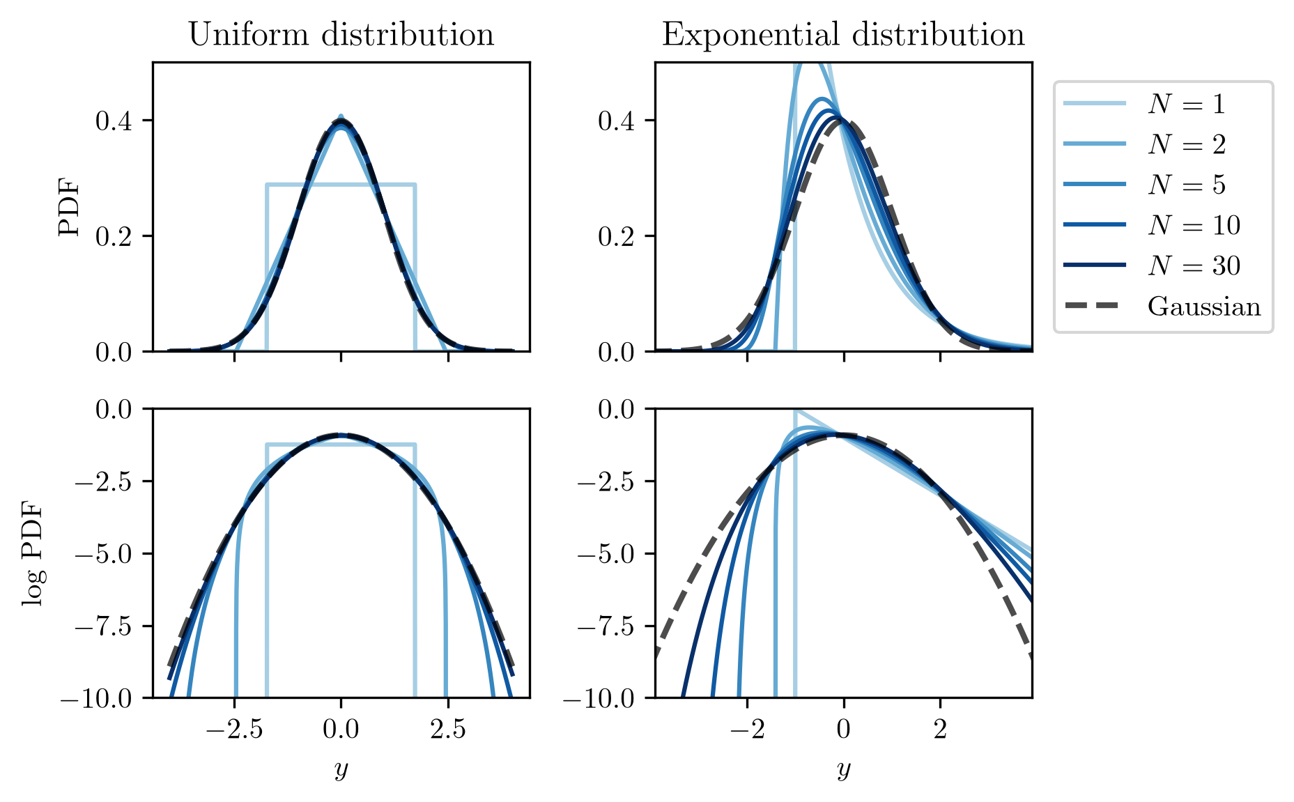
Normalized sums of uniform (left) and exponential (right) draws, on linear (top) and log (bottom) scales.

 

A Gaussian model that is excellent near the mean can be badly wrong far out, and a detector’s false-alarm rate lives far out. Check the approximation where you will use it.

What a digit of \(\pi\) costs

The Monte Carlo estimate is an average of Bernoulli\((\pi/4)\) draws, so by the central limit theorem \[4\,\overline X_N\approx\Gauss\!\paren{\pi,\frac{2.70}{N}},\qquad \text{standard error}=\frac{1.64}{\sqrt N}.\]

At \(N=10^4\) the estimate lies within \(\pm0.032\) of \(\pi\) about 95% of the time. Chebyshev could only promise \(\pm0.1\).

Four correct decimals cost \(N\sim10^8\). The same \(1/\sqrt N\) prices every average in this course: an estimated mean, a sample correlation, a measured spectrum.

Back to the microphone

The self-noise is the sum of an enormous number of tiny, independent contributions: thermal motion of charges in the capsule and the electronics. Their sum must be Gaussian, whatever each contribution looks like, and it is what the histogram showed.

The licence for the rest of the course Model the noise as Gaussian and carry only its mean and variance, as long as it really is many small independent causes.

When the assumption fails: a few large causes

Rustling paper is also noise, but it is made of a few large clicks, not many small ones.

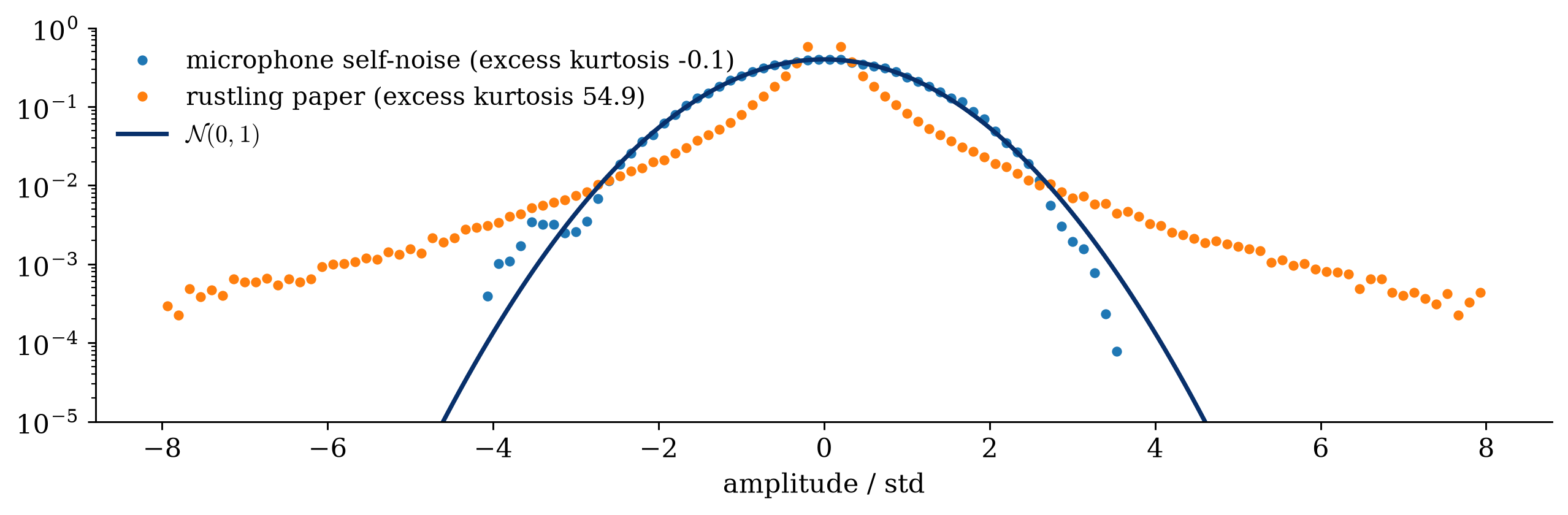
Figure 3: Log-density of the two recordings, each normalized to unit variance, against the Gaussian.

Same variance, wildly different tails. The central limit theorem needs many contributions, none of them dominant; a handful of big events is exactly the case it does not cover.

When the assumption fails: no variance at all

The Cauchy law Bell-shaped, symmetric about \(0\), and with no finite variance. The average of \(N\) Cauchy draws is again Cauchy, with the same width.

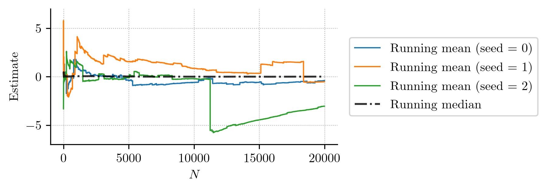
Running averages of Cauchy draws for three seeds, and the running median.

Averaging accomplishes nothing: one large draw undoes all the others. The median settles. The finite variance in the theorem is not a technicality.

Recap

This week

1. A random variable is a map; its law is a density, and two moments, mean and variance, summarize it. The mean is the best constant guess, and the variance is what is left over.

2. For independent variables, means and variances add. An average of \(N\) has variance \(\sigma_X^2/N\): error falls as \(1/\sqrt N\), and counting estimates probabilities, CDFs and densities.

3. Sums of many small independent effects are Gaussian, whatever each effect looks like. That is why noise is Gaussian, and why two moments are enough. It fails for a few large events and for laws without a variance, and it is weakest in the tails.