Linear Optimal Filtering
Estimating one process from another
Observation → desired
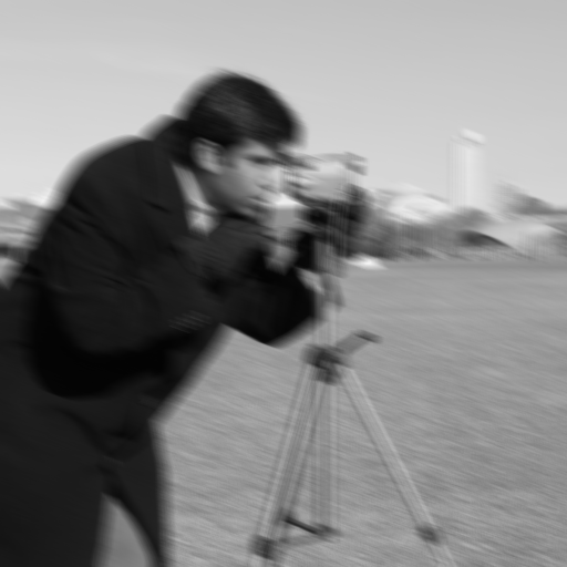
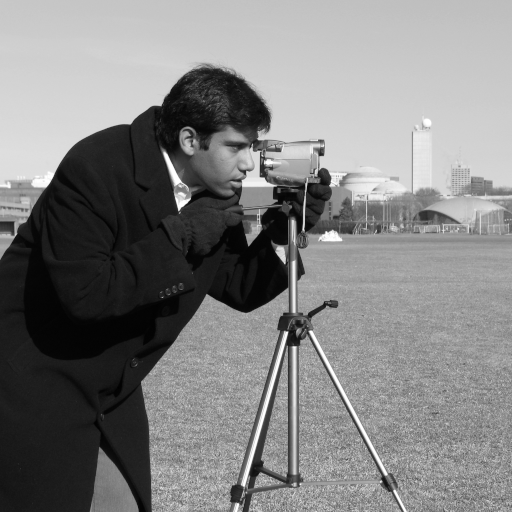
The filter estimates the desired process \(Y\) from the observation \(X\) — same idea, different signals:
Observation \(X\)
Noisy speech
Motion-blurred image
Desired \(Y\)
Clean speech
Sharp image
Observation → desired
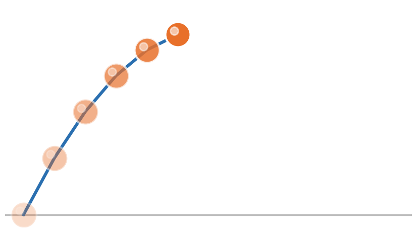
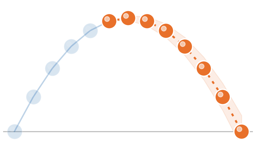
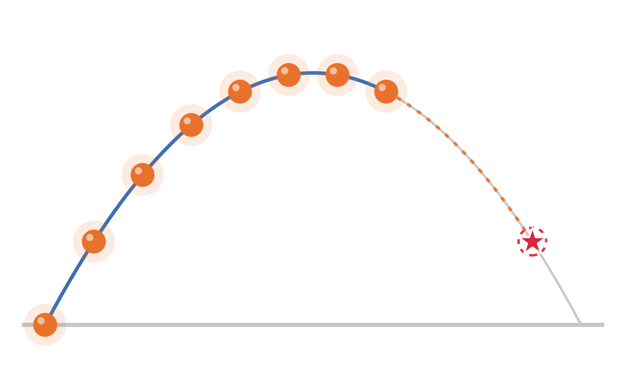
A ballistic flight — predict where the ball is going from where it has been:
Observation \(X\) — the launch
A few measured time steps of the trajectory
Desired \(Y\) — the future
Extrapolated steps ahead (dotted)
From regression to filtering
\[
% Number sets
\newcommand{\Nat}{\mathbb{N}}
\newcommand{\Integer}{\mathbb{Z}}
\newcommand{\Real}{\mathbb{R}}
\newcommand{\Complex}{\mathbb{C}}
% Operators
\newcommand{\SNR}{\operatorname{SNR}}
\newcommand{\tr}{\operatorname{tr}}
\newcommand{\re}{\operatorname{Re}}
\newcommand{\im}{\operatorname{Im}}
\newcommand{\sign}{\operatorname{sign}}
\newcommand{\rect}{\operatorname{rect}}
\newcommand{\sinc}{\operatorname{si}}
\newcommand{\erf}{\operatorname{erf}}
\newcommand{\erfc}{\operatorname{erfc}}
\newcommand{\kurt}{\operatorname{kurt}}
\newcommand{\diag}{\operatorname{diag}}
\newcommand{\MSE}{\operatorname{MSE}}
\newcommand{\argmin}{\operatorname*{argmin}}
\newcommand{\argmax}{\operatorname*{argmax}}
\newcommand{\bias}{\operatorname{bias}}
\newcommand{\Bin}{\operatorname{Bin}}
% Delimiters
\newcommand{\paren}[1]{\left(#1\right)}
\newcommand{\bracket}[1]{\left[#1\right]}
\newcommand{\set}[1]{\left\{#1\right\}}
\newcommand{\abs}[1]{\left\lvert #1 \right\rvert}
\newcommand{\norm}[1]{\left\lVert #1 \right\rVert}
\newcommand{\ip}[1]{\left\langle #1 \right\rangle}
% Notation
\newcommand{\dd}{\,\mathrm{d}}
\newcommand{\tran}{^{\top}}
\newcommand{\conv}{\ast}
\newcommand{\conj}{^{*}}
\newcommand{\herm}{^{\mathsf{H}}}
\newcommand{\opt}{_{\star}}
% Expectation and variance
% \newcommand{\E}[1]{\mathbb{E}\!\left[#1\right]}
\newcommand{\E}[2][]{\mathbb{E}_{#1}\!\left[#2\right]}
\newcommand{\Var}[1]{\mathbb{V}\!\left[#1\right]}
% Distributions
\newcommand{\Gauss}{\mathcal{N}}
\newcommand{\Uniform}{\mathcal{U}}
\newcommand{\FT}{\mathcal{F}}
% Probability
\newcommand{\Prob}[1]{\mathbb{P}\!\left(#1\right)}
% Misc
\newcommand{\bsy}[1]{\boldsymbol{#1}}
\newcommand{\calR}{\mathcal{R}}
\newcommand{\calC}{\mathcal{C}}
\]
In regression we predicted a scalar \(Y\) from a vector of observations \(\mathbf{X}\in\Real^K\) :
\[
\widehat{Y} = \mathbf{h}\tran\mathbf{X},
\qquad
\mathbf{h}\opt = \mathbf{R}_{XX}^{-1}\mathbf{r}_{YX}
\]
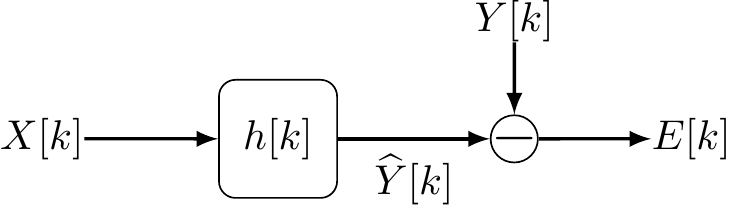
Now the data is a single observation process \(X[k]\) , and we estimate a desired process \(Y[k]\) .
The observation vector is a sliding window of the input process:
\[
\small
\mathbf{X}[k] = \big(X[k],\,X[k-1],\,\ldots,\,X[k-(L-1)]\big)
\]
A linear estimation over that window is a filter — the weights are the impulse response \(h\) :
\[
\widehat{Y}[k] = \mathbf{h}\tran\mathbf{X}[k] = \sum_{\lambda} h[\lambda]\,X[k-\lambda] = (h \conv X)[k]
\]
Building the picture
Before the algebra, build the intuition graphically — what we estimate, and why we may estimate it from a single record.
a window of the observation \(X\) predicting the current value of \(Y\)
three realizations of the same process, and what changes when we slide the window
stacking windows into a least-squares fit — and what overfits
stationarity : the statistics we regress on do not depend on where the window sitsergodicity : so we can estimate them from one time series
→ Demo: From regression to filtering
Normal equations
For a window of length \(L=3\) , \(\;\mathbf{X}=\big(X_0,X_1,X_2\big)\tran\) with \(X_i\equiv X[k-i]\) and \(Y\equiv Y[k]\) , the MMSE weights solve \(\mathbf{R}_{XX}\,\mathbf{h}=\mathbf{r}_{YX}\) written out elementwise:
\[
\small
\underbrace{\begin{pmatrix}
\E{X_0 X_0} & \E{X_0 X_1} & \E{X_0 X_2}\\[2pt]
\E{X_1 X_0} & \E{X_1 X_1} & \E{X_1 X_2}\\[2pt]
\E{X_2 X_0} & \E{X_2 X_1} & \E{X_2 X_2}
\end{pmatrix}}_{\mathbf{R}_{XX}}
\begin{pmatrix} h_0\\ h_1\\ h_2 \end{pmatrix}
=
\underbrace{\begin{pmatrix} \E{Y X_0}\\ \E{Y X_1}\\ \E{Y X_2} \end{pmatrix}}_{\mathbf{r}_{YX}}
\quad\Longrightarrow\quad
\boxed{\,\mathbf{h}\opt = \mathbf{R}_{XX}^{-1}\,\mathbf{r}_{YX}\,}
\]
For jointly weakly stationary \(X,Y\) every entry \(\E{X_i X_j}=R_{XX}[\,i-j\,]\) depends only on the lag, so \(\mathbf{R}_{XX}\) is Toeplitz .
\[
\small
\begin{pmatrix}
R_{XX}[\,0\,] & R_{XX}[\,-1\,] & R_{XX}[\,-2\,]\\[2pt]
R_{XX}[\,1\,] & R_{XX}[\,0\,] & R_{XX}[\,-1\,]\\[2pt]
R_{XX}[\,2\,] & R_{XX}[\,1\,] & R_{XX}[\,0\,]
\end{pmatrix}
\begin{pmatrix} h_0\\ h_1\\ h_2 \end{pmatrix}
=
\begin{pmatrix} R_{YX}[0]\\ R_{YX}[1]\\ R_{YX}[2] \end{pmatrix}
\]
Orthogonality principle
Minimize the mean squared error \(J(h)=\E{E^2[k]}\) with \(E[k]=Y[k]-\widehat{Y}[k]\) . Using \(\partial E[k]/\partial h[\kappa]=-X[k-\kappa]\) :
\[
\frac{\partial J}{\partial h[\kappa]} = -2\,\E{E[k]\,X[k-\kappa]} \stackrel{!}{=} 0
\]
Orthogonality principle At the optimum, the minimum error is orthogonal to every observation that enters the estimate: \[
E\opt[k] \perp X[k-\kappa]
\quad\Longleftrightarrow\quad
\E{E\opt[k]\,X[k-\kappa]} = 0
\qquad \forall \kappa
\]
The same MMSE normal equation as in regression: the residual is what the filter cannot explain.
Linear prediction
The desired process is the same signal one step ahead. Predict \(X[k]\) from its own past:
\[
\widehat{X}[k] = \sum_{i=1}^{L} h[i]\,X[k-i],
\qquad
E[k] = X[k]-\widehat{X}[k]
\]
For a length-\(L=3\) predictor this gives the Yule–Walker
\[
\small
\underbrace{\begin{pmatrix}
R_{XX}[\,0\,] & R_{XX}[\,-1\,] & R_{XX}[\,-2\,]\\[2pt]
R_{XX}[\,1\,] & R_{XX}[\,0\,] & R_{XX}[\,-1\,]\\[2pt]
R_{XX}[\,2\,] & R_{XX}[\,1\,] & R_{XX}[\,0\,]
\end{pmatrix}}_{\mathbf{R}_{XX}}
\begin{pmatrix} h[1]\\ h[2]\\ h[3] \end{pmatrix}
=
\underbrace{\begin{pmatrix} R_{XX}[1]\\ R_{XX}[2]\\ R_{XX}[3] \end{pmatrix}}_{\mathbf{r}_{XX}}
\]
Innovations
With the infinite-past causal optimal linear predictor, the residual \(E\opt[k]\) is called the innovation
\[
\widehat{X}[k]
=
\sum_{i=1}^{\infty} h\opt[i]\,X[k-i],
\qquad
E\opt[k]=X[k]-\widehat{X}[k].
\]
By the orthogonality principle, the minimum-error residual is orthogonal to every past sample:
\[
\E{E\opt[k]\,X[k-\kappa]}=0,
\qquad \kappa=1,2,\ldots
\]
As a consequence, the residual is weakly white, i.e., for \(\kappa>0\)
\[
\E{E\opt[k]\,E\opt[k-\kappa]}= \E{E\opt[k]\,(X[k-\kappa] - \sum_{i=1}^{\infty} h\opt[i]\,X[k-i-\kappa])} = 0 .
\]
Linear predictive coding (LPC): transmitter and receiver
Before transmitting a signal, linear prediction removes redundancy from non-white random processes.
The transmitted signal is the innovation \(E[k]\) (white) plus the filter coefficients \(h[i]\) (small, fixed).
General case: the Wiener–Hopf equation
Let the filter be infinitely long (and possibly noncausal): \(\;\widehat{Y}[k]=\sum_{\lambda=-\infty}^{\infty} h[\lambda]X[k-\lambda]\) .
Orthogonality \(\E{E\opt[k]X[k-\kappa]}=0\) holds for all \(\kappa\) , giving the Wiener–Hopf equation
\[
R_{YX}[\kappa] = \sum_{\lambda=-\infty}^{\infty} h\opt[\lambda]\,R_{XX}[\kappa-\lambda] = (h\opt \conv R_{XX})[\kappa]
\qquad \forall \kappa
\]
This is the FIR normal equation \(\mathbf{R}_{XX}\mathbf{h}=\mathbf{r}_{YX}\) taken to infinite length — a convolution on the right-hand side.
A convolution that holds for all lags is begging for a Fourier transform.
Manipulating the PSD
LTI filtering
\(Y=h\conv X\) \(\abs{H(e^{j\Omega})}^2\,S_{XX}\) \(H(e^{j\Omega})\,S_{XX}\)
scaling
\(Y=aX\) \(\abs{a}^2\,S_{XX}\) \(a\,S_{XX}\)
delay
\(Y[k]=X[k-k_0]\) \(S_{XX}\) \(e^{-j\Omega k_0}\,S_{XX}\)
sum (general)
\(Y=X+U\) \(S_{XX}+S_{UU} + 2\,\re\{S_{UX}\}\) \(S_{XX} + S_{UX}\)
sum (\(X \perp U\) )
\(Y=X+U\) \(S_{XX}+S_{UU}\) \(S_{XX}\)
Frequency domain
Take the DTFT of the Wiener–Hopf equation — the convolution becomes a product:
\[
\boxed{\,H\opt(e^{j\Omega}) = \frac{S_{YX}(e^{j\Omega})}{S_{XX}(e^{j\Omega})}\,}
\]
White observation \(S_{XX}[e^{j\Omega}]=R_0\) collapses the solve to a scaling: \[\;H\opt(e^{j\Omega}) = S_{YX}(e^{j\Omega})/R_0\]
The residual error power of the optimal filter:
\[
\E{E\opt^2[k]}
= \frac{1}{2\pi}\int_0^{2\pi}
\left[\,S_{YY}(e^{j\Omega}) - \frac{\big|S_{YX}(e^{j\Omega})\big|^2}{S_{XX}(e^{j\Omega})}\,\right]\dd\Omega
\]
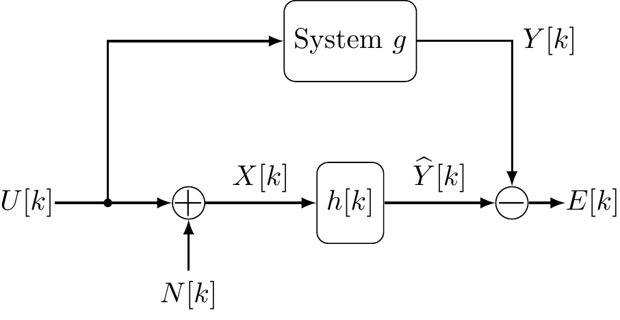
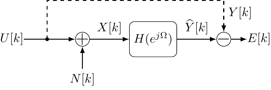
Standard model: signal in noise
Observation is signal plus noise, \(\;X[k] = U[k] + N[k]\) (with \(U\perp N\) ):
\[
H\opt(e^{j\Omega}) = \frac{S_{YX}(e^{j\Omega})}{S_{XX}(e^{j\Omega})}
= G(e^{j\Omega})\,
\frac{S_{UU}(e^{j\Omega})}{S_{UU}(e^{j\Omega}) + S_{NN}(e^{j\Omega})}
\]
One ballistic flight - three tasks
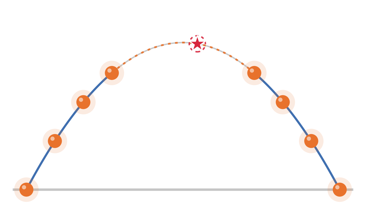
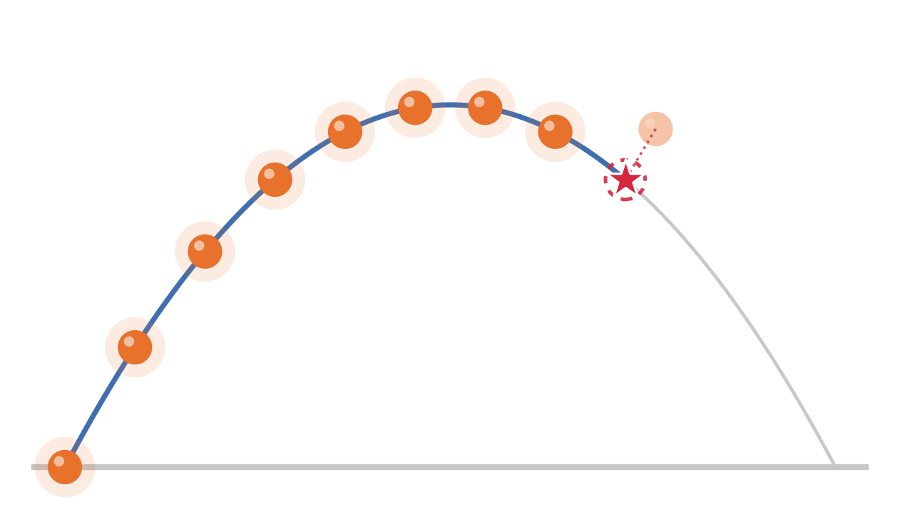
The same trajectory, differing only in where the estimate (★ ) sits relative to the measurements (● ):
smoothing — \(k_0>0\)
A step is missing — estimate it from measurements before and after .
filtering — \(k_0=0\)
Clean up the current noisy measurement using the present and past.
prediction — \(k_0<0\)
Extrapolate a future step from the record so far.
Smoothing, filtering, prediction
A pure delay \(g[k]=\delta[k-k_0]\) (so \(Y[k]=U[k-k_0]\) ) gives three tasks:
\(k_0>0\) smoothing — estimate a past valuepast and future \(X\)
\(k_0=0\) filtering — estimate the current valuecausal: present + past
\(k_0<0\) prediction — estimate a future valuecausal: present + past
→ Demo: Smoothing / Filtering / Prediction
Noise suppression
Take the clean component as desired, \(Y=U\) , with \(g=\delta\) (so \(G=1\) ):
\[
H\opt(e^{j\Omega}) =
\frac{S_{UU}(e^{j\Omega})}{S_{UU}(e^{j\Omega}) + S_{NN}(e^{j\Omega})}
\]
In practice \(S_{UU}\) is unknown but a noise estimate \(S_{NN}\) is available:
\[
\boxed{\,H\opt(e^{j\Omega}) = \frac{S_{XX}(e^{j\Omega}) - S_{NN}(e^{j\Omega})}{S_{XX}(e^{j\Omega})}\,}
\]
Speech enhancement
\[
H\opt(e^{j\Omega}) = \frac{S_{XX}(e^{j\Omega}) - S_{NN}(e^{j\Omega})}{S_{XX}(e^{j\Omega})}
\]
The gain is \(\approx 1\) where signal dominates, \(\approx 0\) where noise dominates — frame-wise speech enhancement .
→ Demo: Single-channel noise suppression
Recap
A filter is multidimensional MMSE over a sliding window — the regression normal equations, indexed by lag.
\(\mathbf{R}_{XX}\mathbf{h}\opt=\mathbf{r}_{YX}\) (Toeplitz)causal FIR Wiener filter
\(\mathbf{R}_{XX}\mathbf{h}\opt=\mathbf{r}_{XX}\) linear predictor (Yule–Walker)
\(R_{YX}=h\opt\conv R_{XX}\) (all lags)Wiener–Hopf equation — time domain (infinite length)
\(H\opt = S_{YX}/S_{XX}\) Wiener–Hopf solved — frequency domain (noncausal)
All under one criterion: minimum mean squared error .
Next : a different question — not what is the signal, but is it there? Detection brings back the likelihood-ratio test — and it hands us a filter.
From detection back to the LRT
We proved that for two simple hypotheses the optimal test is the likelihood-ratio test :
\[
\Lambda(\mathbf{x}) = \frac{f_{\mathbf{X}\mid H_1}(\mathbf{x})}{f_{\mathbf{X}\mid H_0}(\mathbf{x})}
\;\underset{H_0}{\overset{H_1}{\gtrless}}\; \eta
\]
Point it at a known signal in noise — a reference \(\mathbf{u}\) (radar echo, sync word, pilot tone) at a known position , present or not, in Gaussian noise \(\mathbf{N}\sim\Gauss(\mathbf{0},\mathbf{R}_{NN})\) :
\[
H_0:\ \mathbf{X}=\mathbf{N}
\qquad\text{vs.}\qquad
H_1:\ \mathbf{X}=\mathbf{u}+\mathbf{N}
\]
The timing is known, so the data is a single length-\(L\) vector \(\mathbf{x}\) — we only decide present or absent .
Looking for a known signal
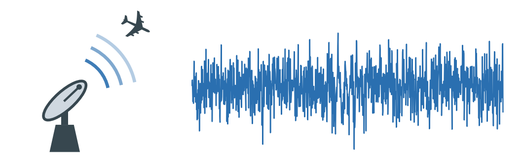
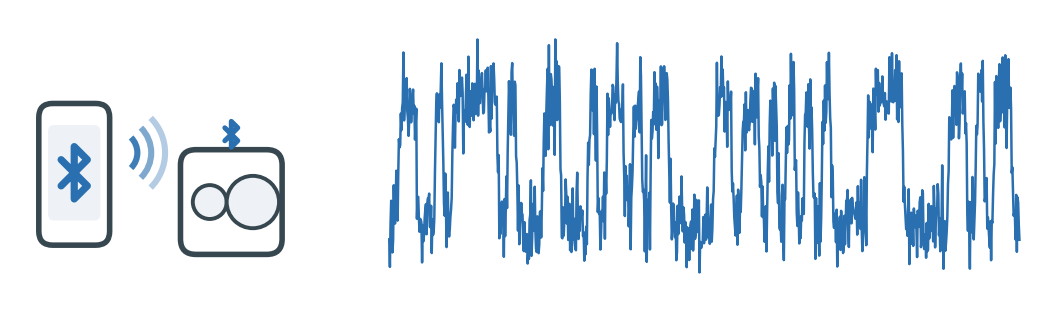
Observation \(X\) — the received scene
Radar / sonar / LiDAR — echoes buried in noise
Bluetooth LE — RF stream from many devices
Template \(u\) — what we look for
The emitted chirp (range \(=\) delay of the match)
The known preamble / access address
A known signal, buried in noise
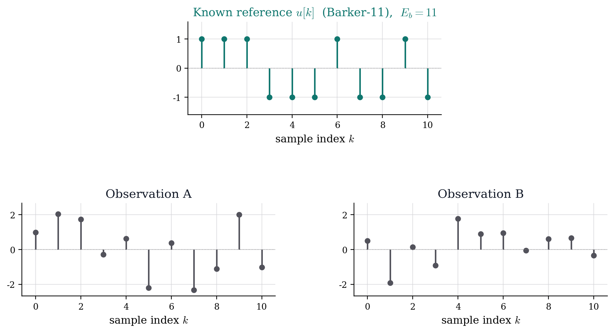
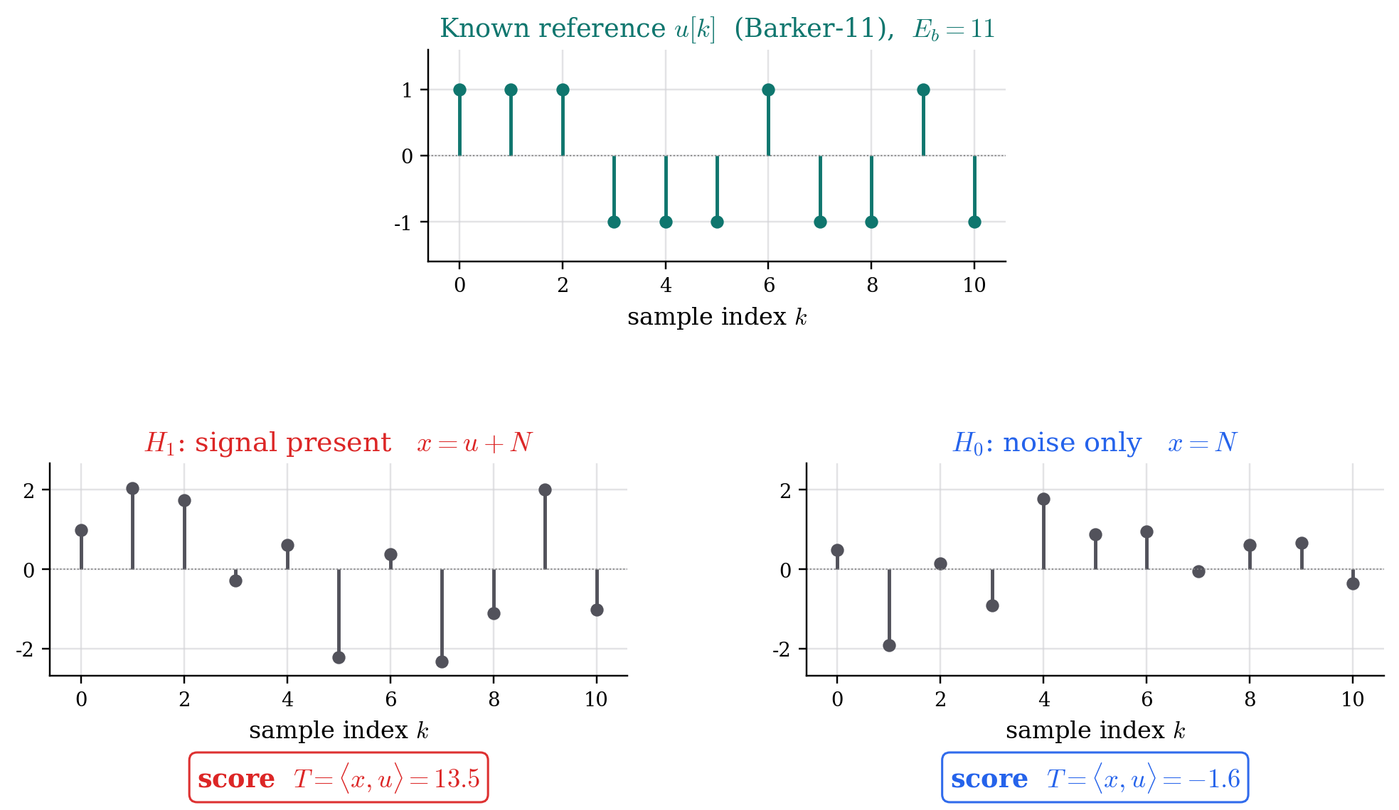
The reference \(\mathbf{u}\) is known exactly ; only its presence is in question. In noise, the two hypotheses produce traces that look alike:
Road 1 — the Gaussian LRT is linear
Both likelihoods are Gaussian, so take the log -ratio — the quadratic-in-\(\mathbf{x}\) terms cancel:
\[
\ln\Lambda(\mathbf{x})
= -\tfrac12(\mathbf{x}-\mathbf{u})\tran\mathbf{R}_{NN}^{-1}(\mathbf{x}-\mathbf{u})
+ \tfrac12\,\mathbf{x}\tran\mathbf{R}_{NN}^{-1}\mathbf{x}
= \mathbf{u}\tran\mathbf{R}_{NN}^{-1}\mathbf{x} - \tfrac12\,\mathbf{u}\tran\mathbf{R}_{NN}^{-1}\mathbf{u}
\]
The constant folds into the threshold. The optimal test thresholds a statistic linear in the data — a filter with weights \(\mathbf{w}=\mathbf{R}_{NN}^{-1}\mathbf{u}\) :
\[
\boxed{\;T(\mathbf{x}) = \mathbf{w}\tran\mathbf{x} = \mathbf{u}\tran\mathbf{R}_{NN}^{-1}\mathbf{x}
\;\underset{H_0}{\overset{H_1}{\gtrless}}\; \gamma\;}
\]
For a Gaussian signal-in-noise problem, the optimal detector is a linear filter .
White noise: correlate with the template
White noise \(\mathbf{R}_{NN}=R_0\,\mathbf{I}\) makes the weights proportional to the signal itself:
\[
T(\mathbf{x}) = \frac{1}{R_0}\,\mathbf{u}\tran\mathbf{x}
= \frac{1}{R_0}\sum_k u[k]\,x[k]
= \frac{1}{R_0}\,\ip{\mathbf{x},\mathbf{u}}
\]
The optimal score is just the correlation of the data with the template — the matched filter .
Noise-free it returns the energy \(\ip{\mathbf{u},\mathbf{u}}=E_b\) ; under \(H_0\) the term \(\ip{\mathbf{N},\mathbf{u}}\) has zero mean. A large score ⇔ the signal is present.
Road 2 — maximum output SNR
The same weights arise with no distributional assumption . Among all linear scores \(T=\mathbf{w}\tran\mathbf{x}\) , which best separates the hypotheses? Maximize the deflection
\[
(d')^{2} = \frac{\big(\E{T\mid H_1}-\E{T\mid H_0}\big)^2}{\Var{T\mid H_0}}
= \frac{(\mathbf{w}\tran\mathbf{u})^2}{\mathbf{w}\tran\mathbf{R}_{NN}\,\mathbf{w}}
\]
Cauchy–Schwarz maximizes this with the same weights \(\mathbf{w}\opt=\mathbf{R}_{NN}^{-1}\mathbf{u}\) :
\[
(d')^{2} = \mathbf{u}\tran\mathbf{R}_{NN}^{-1}\mathbf{u}
\quad\xrightarrow{\ \text{white}\ }\quad
d' = \sqrt{E_b/R_0},\qquad E_b=\sum_k u^2[k]
\]
Only the signal energy matters, not the shape. In white noise the deflection separates \(H_0:T\sim\Gauss(0,R_0E_b)\) from \(H_1:T\sim\Gauss(E_b,R_0E_b)\) — more energy ⇒ better-separated hypotheses ⇒ a better ROC .
Derivation: whiten first, then Cauchy–Schwarz
Since \(\mathbf{R}_{NN}\succ 0\) , insert \(\mathbf{R}_{NN}^{1/2}\mathbf{R}_{NN}^{-1/2}\) and substitute \(\mathbf{a}=\mathbf{R}_{NN}^{1/2}\mathbf{w}\) , \(\;\mathbf{b}=\mathbf{R}_{NN}^{-1/2}\mathbf{u}\) :
\[
\mathbf{w}\tran\mathbf{u} = (\mathbf{R}_{NN}^{1/2}\mathbf{w})\tran(\mathbf{R}_{NN}^{-1/2}\mathbf{u})
= \mathbf{a}\tran\mathbf{b},
\qquad
\mathbf{w}\tran\mathbf{R}_{NN}\,\mathbf{w} = \norm{\mathbf{a}}^2
\]
The deflection becomes a pure Cauchy–Schwarz shape, with a bound that no longer depends on \(\mathbf{w}\) :
\[
(d')^{2} = \frac{(\mathbf{a}\tran\mathbf{b})^2}{\norm{\mathbf{a}}^2}
\;\le\; \norm{\mathbf{b}}^2 = \mathbf{u}\tran\mathbf{R}_{NN}^{-1}\mathbf{u}
\]
Equality holds exactly when \(\mathbf{a}=c\,\mathbf{b}\) , i.e. \(\mathbf{R}_{NN}^{1/2}\mathbf{w}=c\,\mathbf{R}_{NN}^{-1/2}\mathbf{u}\) ; multiply by \(\mathbf{R}_{NN}^{-1/2}\) :
\[
\boxed{\;\mathbf{w}\opt = \mathbf{R}_{NN}^{-1}\mathbf{u}\;}
\]
The scale \(c\) is free — \((d')^2\) is invariant to \(\mathbf{w}\mapsto c\,\mathbf{w}\) .
The two roads meet
The matched filter is optimal in two different senses :
maximize output SNR / deflection among linear filters (Cauchy–Schwarz — no distribution assumed)
the Neyman–Pearson detector for Gaussian noise (the LRT)
They coincide because, for Gaussian noise, the log-likelihood ratio is linear in the data — so the best linear score is already the best possible test.
Drop Gaussianity and they split: the matched filter still maximizes SNR, but the optimal detector becomes nonlinear.
Unknown timing: a bank of matched filters
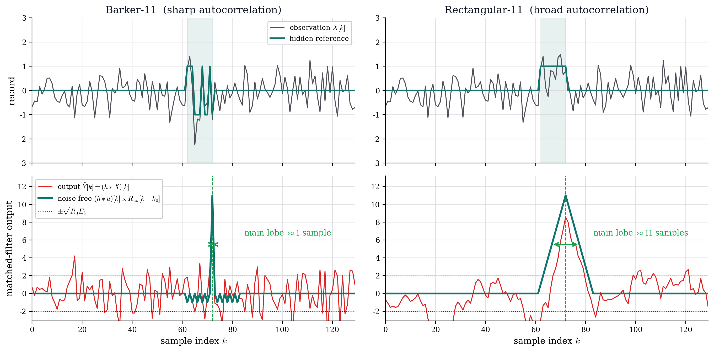
So far the timing was known. Now the arrival time \(k_0\) is unknown , and the data is a running stream \(X[k]\) — not one aligned vector. So test every shift: for each candidate \(k_0\) ,
\[
T_{k_0} = \ip{\mathbf{X},\mathbf{u}_{k_0}} = \sum_k u[k-k_0]\,X[k]
\]
Evaluating this for all \(k_0\) at once is a bank of matched filters — a convolution of the random observation \(X[k]\) with the time-reversed reference — hence matched :
\[
\widehat{Y}[k] = \sum_{\lambda} h\opt[\lambda]\,X[k-\lambda] = (h\opt\conv X)[k],
\qquad
h\opt[k]\propto u[-k]
\]
With no noise, the filter returns the reference’s autocorrelation, shifted to the arrival and peaking at \(k_0\) :
\[
\widehat{Y}[k]\big|_{\text{noise-free}}\propto R_{uu}[k-k_0]
\]
Colored noise: prewhiten, then match
For colored noise the optimal weights \(\mathbf{w}=\mathbf{R}_{NN}^{-1}\mathbf{u}\) are the same idea with a whitening step. In the frequency domain it is a single filter with a delay:
\[
H\opt(e^{j\Omega}) = \frac{U\conj(e^{j\Omega})\,e^{-j\Omega k_0}}{S_{NN}(e^{j\Omega})}
\]
\(1/S_{NN}\) — prewhitening : discount frequencies where noise dominates\(U\conj(e^{j\Omega})\,e^{-j\Omega k_0}\) — matching : correlate with the (delayed) reference
Two criteria, two filters
min MSE Wiener filter \(H\opt = S_{YX}/S_{XX}\)
what is the signal? (estimation)
max output SNR matched filter \(h\opt\propto u[-k]\)
is the signal there? (detection)