The Wiener Filter

The normal equations become a convolution

Speech in noise

\[ % Number sets \newcommand{\Nat}{\mathbb{N}} \newcommand{\Integer}{\mathbb{Z}} \newcommand{\Real}{\mathbb{R}} \newcommand{\Complex}{\mathbb{C}} % Operators \newcommand{\SNR}{\operatorname{SNR}} \newcommand{\tr}{\operatorname{tr}} \newcommand{\re}{\operatorname{Re}} \newcommand{\im}{\operatorname{Im}} \newcommand{\sign}{\operatorname{sign}} \newcommand{\rect}{\operatorname{rect}} \newcommand{\sinc}{\operatorname{si}} \newcommand{\erf}{\operatorname{erf}} \newcommand{\erfc}{\operatorname{erfc}} \newcommand{\kurt}{\operatorname{kurt}} \newcommand{\diag}{\operatorname{diag}} \newcommand{\MSE}{\operatorname{MSE}} \newcommand{\argmin}{\operatorname*{argmin}} \newcommand{\argmax}{\operatorname*{argmax}} \newcommand{\bias}{\operatorname{bias}} \newcommand{\Bin}{\operatorname{Bin}} % Delimiters \newcommand{\paren}[1]{\left(#1\right)} \newcommand{\bracket}[1]{\left[#1\right]} \newcommand{\set}[1]{\left\{#1\right\}} \newcommand{\abs}[1]{\left\lvert #1 \right\rvert} \newcommand{\norm}[1]{\left\lVert #1 \right\rVert} \newcommand{\ip}[1]{\left\langle #1 \right\rangle} % Notation \newcommand{\dd}{\,\mathrm{d}} \newcommand{\tran}{^{\top}} \newcommand{\conv}{\ast} \newcommand{\conj}{^{*}} \newcommand{\herm}{^{\mathsf{H}}} \newcommand{\opt}{^{\star}} % Expectation and variance % \newcommand{\E}[1]{\mathbb{E}\!\left[#1\right]} \newcommand{\E}[2][]{\mathbb{E}_{#1}\!\left[#2\right]} \newcommand{\Var}[1]{\mathbb{V}\!\left[#1\right]} % Distributions \newcommand{\Gauss}{\mathcal{N}} \newcommand{\Uniform}{\mathcal{U}} \newcommand{\FT}{\mathcal{F}} % Probability \newcommand{\Prob}[1]{\mathbb{P}\!\left(#1\right)} % Misc \newcommand{\bsy}[1]{\boldsymbol{#1}} \newcommand{\calR}{\mathcal{R}} \newcommand{\calC}{\mathcal{C}} \]

Can a filter pull the speech out?

Speech with a tonal beep on top, and the same speech next to a blender:

We want a filter \(h\) whose output \(\widehat Y=h*X\) is as close as possible, in mean square, to the clean speech \(Y\).

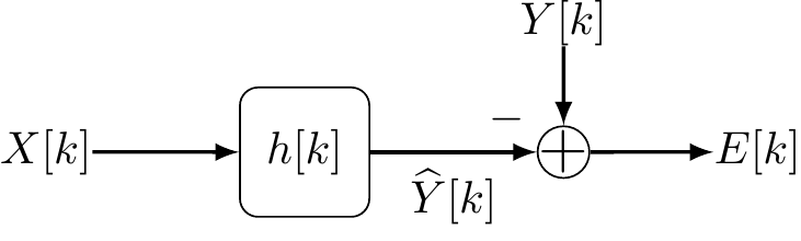
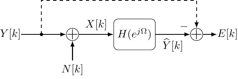
The observation \(X\) is filtered to approximate the desired \(Y\); the error \(E\) is what \(h\) minimizes.

Estimation-as-projection once more, with the observations now a whole process.

By the end of the week the same answer will also be a system identifier, a predictor, a smoother, a deblurrer, a pulse detector and a broadband beamformer.

The plan for the week

The Wiener–Hopf equation. The orthogonality principle on a process: the normal equations become a convolution, and in frequency a ratio of spectra.

One equation, many right-hand sides. System identification, prediction, filtering and smoothing, deconvolution, the running matched filter, broadband arrays: the same Toeplitz system with a different target.

In the notes The Wiener Filter · System Identification · Estimation Within One Process · Filtering and Smoothing · Inverse Problems: Wiener Deconvolution · The Matched Filter · Space–Time and Broadband Array Processing

The Wiener–Hopf equation

The normal equations, as a convolution

Orthogonality: the error must be uncorrelated with every observation sample, \(\E{E[k]\,X\conj[k-\kappa]}=0\) for all \(\kappa\). With stationarity:

Wiener–Hopf equation \[R_{YX}[\kappa]=\sum_\lambda h\opt[\lambda]\,R_{XX}[\kappa-\lambda]=(h\opt*R_{XX})[\kappa].\]

Exactly \(\mathbf w\herm\mathbf R_{\mathbf{XX}}=\mathbf r_{\mathbf{YX}}\), the normal equations for the map: the Gram matrix is the Toeplitz autocorrelation, and \(h[\lambda]=w_\lambda\conj\).

Nothing new was derived. A matrix equation became a convolution because the index set grew.

In frequency, a ratio

The Fourier transform diagonalizes the convolution:

Non-causal Wiener filter \[H\opt(e^{j\Omega})=\frac{S_{YX}(e^{j\Omega})}{S_{XX}(e^{j\Omega})},\qquad S_{EE}=S_{YY}-\frac{\abs{S_{YX}}^2}{S_{XX}}=S_{YY}\paren{1-\abs{\rho_{YX}(e^{j\Omega})}^2}.\]

One scalar normal equation per frequency, because the complex exponentials are the eigenvectors of every stationary process. The error spectrum is the target spectrum times one minus the coherence.

For a white observation, \(R_{XX}=R_0\delta\), the filter is just \(h\opt=R_{YX}/R_0\): correlate with the target. That is why whitening the observation first is such a common step.

The phase is not free

Estimation determines phase The Wiener solution fixes \(H\opt\) completely: magnitude and phase at every frequency. The numerator \(S_{YX}\) is a cross-spectrum, so it carries the delay between observation and target.

Contrast spectral factorization: an auto-spectrum \(\abs{H}^2\) has thrown its phase away, and minimum phase had to be imposed.

With a finite window

A filter of \(L\) taps keeps the Wiener–Hopf equation over its support only:

FIR Wiener filter \[\begin{bmatrix}R_{XX}[0]&R_{XX}[-1]&\cdots\\R_{XX}[1]&R_{XX}[0]&\cdots\\ \vdots&&\ddots\end{bmatrix} \begin{bmatrix}h\conj[0]\\h\conj[1]\\ \vdots\end{bmatrix} =\begin{bmatrix}R_{XY}[0]\\R_{XY}[1]\\ \vdots\end{bmatrix} .\]

An \(L\times L\) Toeplitz system, fixed by \(L\) correlation lags. Levinson–Durbin solves it in \(O(L^2)\) instead of \(O(L^3)\).

→ Demo: from regression to filtering

Denoising

Pass what is signal

The clean process is observed as \(X=Y+N\) and filtered to approximate \(Y\).

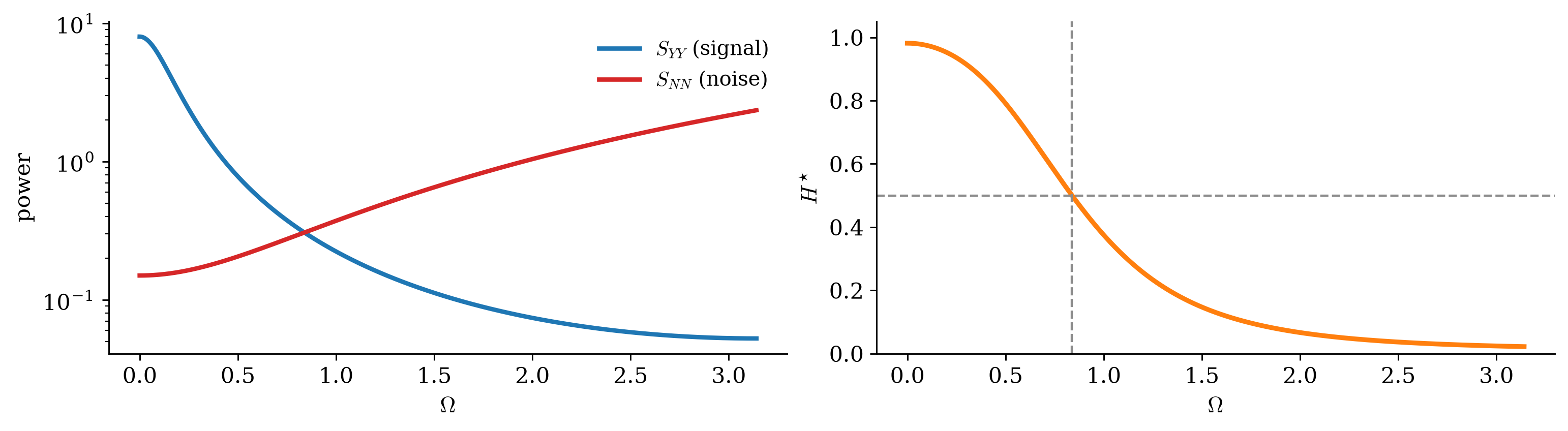
With \(Y\) and \(N\) uncorrelated, \(S_{YX}=S_{YY}\) and \(S_{XX}=S_{YY}+S_{NN}\): \[H\opt=\frac{S_{YY}}{S_{YY}+S_{NN}}\in[0,1] .\]

The scalar shrinkage of the Bayesian week, once per frequency: the fraction of the observed power at \(\Omega\) that is signal.

The gain, drawn

Figure 1: A low-pass signal spectrum against rising noise, and the Wiener gain. The gain crosses 1/2 where the spectra cross.

The noise floor sits in the denominator, so the filter never divides by anything near zero.

Where the error lives

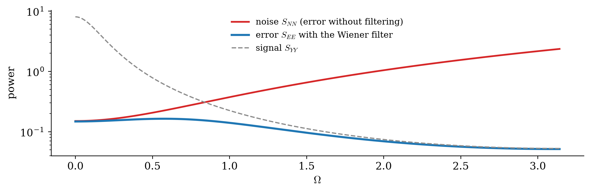
Figure 2: The same two spectra: the error spectrum S_EE = S_YY S_NN / (S_YY + S_NN) of the Wiener filter, against the noise it started from.

\(S_{EE}\) is the smaller of signal and noise, roughly, at every frequency: where noise dominates the filter gives up the signal, where signal dominates it keeps the noise. The total error is the area under the blue curve.

The speech, filtered

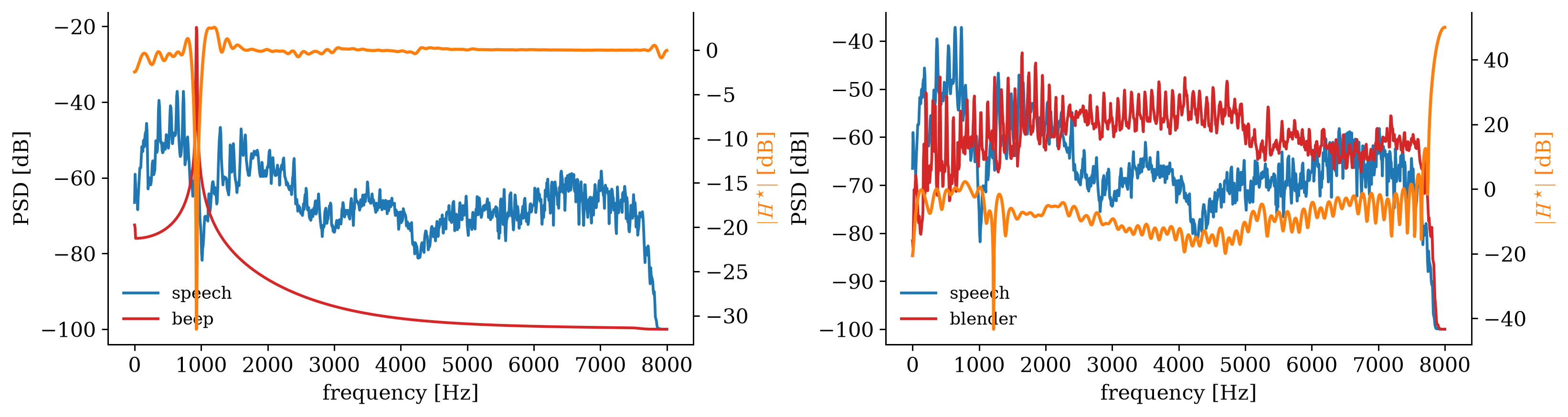
Figure 3: Left: speech and beep spectra, and the Wiener filter’s response (a 128-tap FIR from the Wiener–Hopf equation). Right: the same for the blender.

SNR improvement: beep 22.5 dB, blender 3.8 dB

Where the statistics come from

The filter needs \(R_{XX}\) and \(R_{YX}\). Here \(R_{XX}\) is estimated from the noisy recording itself, by time averages, which is ergodicity at work.

\(R_{YX}\) needs the clean target: two ways out

• a model: \(S_{YX}=S_{YY}\), \(S_{XX}=S_{YY}+S_{NN}\) for uncorrelated noise, \(S_{NN}\) measured in speech pauses;
• a training set of clean and noisy pairs.

Every practical noise suppressor is one of these two.

What decides whether it helps

• Narrowband interference: the beep sits in a few bands; the filter notches them.
• Broadband interference: the blender overlaps the speech almost everywhere.

No LTI filter separates what the spectra do not The design is optimal both times; \(S_{YY}(1-\abs{\rho_{YX}}^2)\) says exactly how much error is unavoidable.

→ Demo: noise suppression and the Wiener gain

System identification

Correlation is the answer

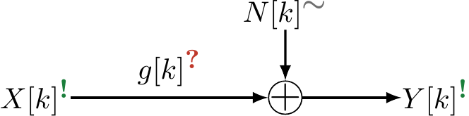
Input and output both observed, noise at the output, the system in between sought.

The unknown is the system \(g\), and the Wiener–Hopf equation reads \(R_{YX}=g*R_{XX}\). Drive it with white input, \(R_{XX}=R_0\delta\), and it collapses: \[g[\kappa]=R_{YX}[\kappa]/R_0 .\] The input–output cross-correlation is the impulse response: nothing solved, nothing inverted.

With a colored input the same measurement is the impulse response convolved with \(R_{XX}\): either whiten the input or solve the Toeplitz system.

Measuring a response

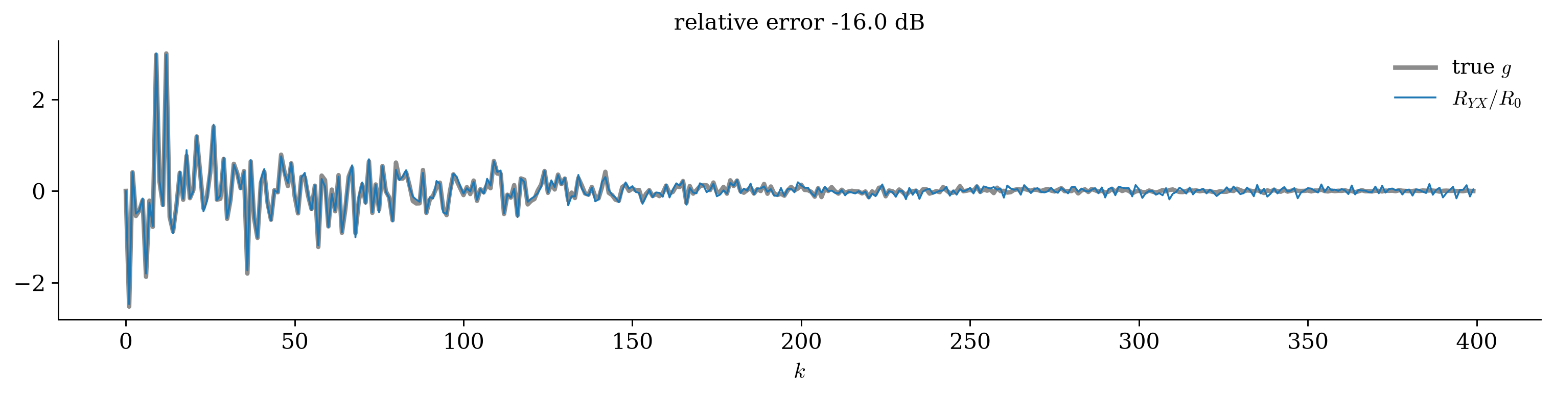
Figure 4: A room-like impulse response, measured by cross-correlating 2 s of white-noise excitation with the noisy output (output SNR 10 dB).

The error falls with the length of the excitation, like any average. This is how the acoustics of a room, a loudspeaker or a channel are measured.

A guitar amp is not linear

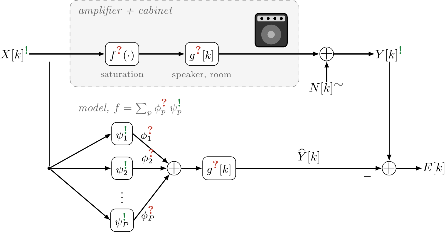
The amp as a saturation \(f\) followed by the cabinet \(g\) (above), and the model: \(f\) expanded in fixed basis functions \(\psi_p\) (below).

Expand \(f=\sum_p \phi_p\psi_p\) and the output is \(\sum_{p,\ell} c_{p\ell}\,\psi_p(X[k-\ell])\) with \(c_{p\ell}=\phi_p\,g[\ell]\): linear in the unknowns. The same normal equations, with \(P\) feature signals as inputs instead of one.

→ Demo: identifying a guitar amp

Estimation within one process

Prediction: the signal as its own target

Predict \(X[k]\) from its own past. The target is a future sample of the observation itself.

The prediction error is white With the whole past available, the optimal one-step prediction error of a regular WSS process is white; the prediction-error filter is a whitening filter.

Why. Each error is orthogonal to the whole past, which contains every earlier error: the errors are the innovations, with power \(\sigma_E^2=\exp\paren{\frac{1}{2\pi}\int\ln S_{XX}\dd\Omega}\).

Prediction and the minimum-phase whitener are one filter: one from a spectrum, one from a past.

Prediction: the signal as its own target

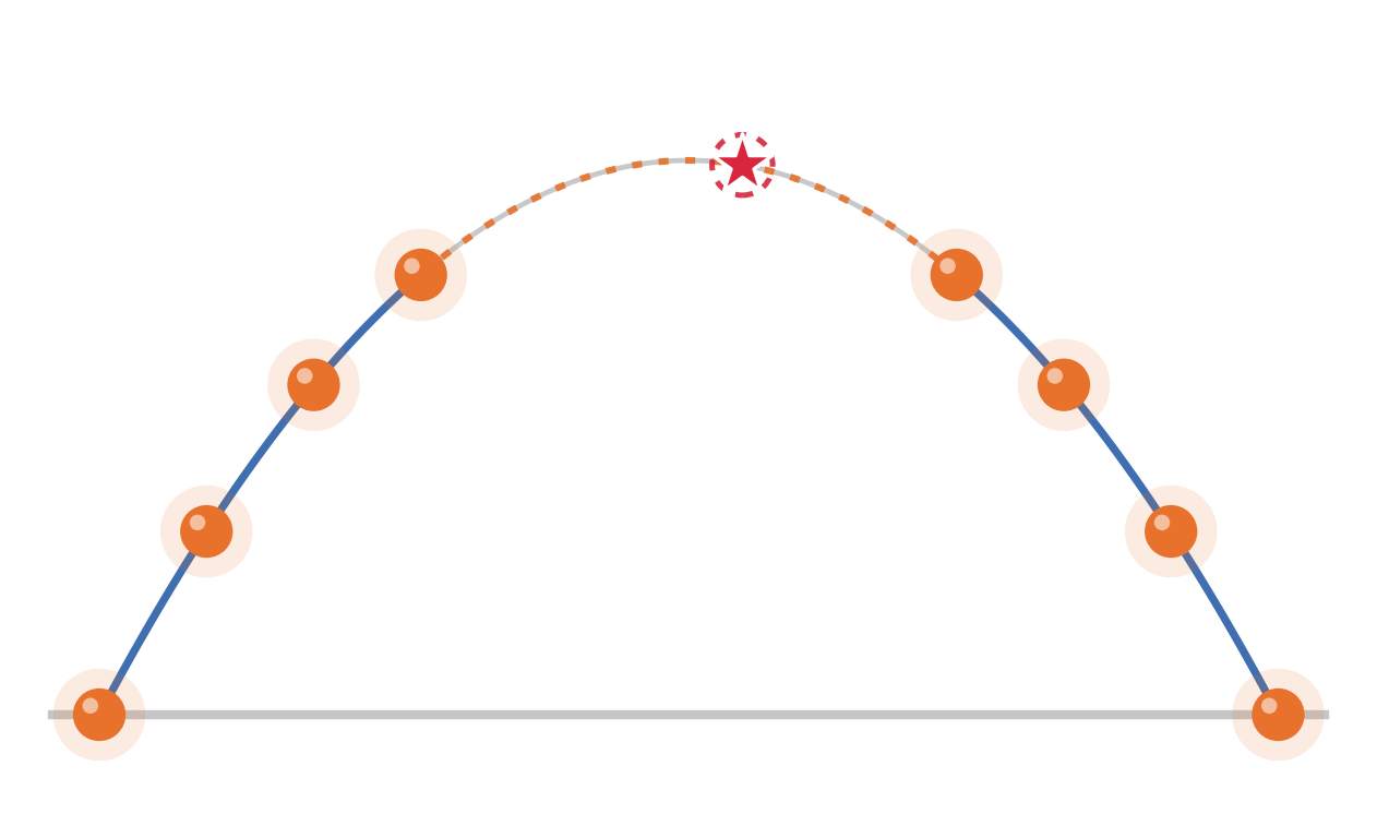
Prediction as a signal flow: no noise, no system, only a delay between the sample sought and the samples in hand.

The finite past: Yule–Walker

With the last \(p\) samples, the normal equations are Toeplitz and fixed by \(p+1\) correlation lags:

Yule–Walker equations \[R_{XX}[l]=-\sum_{i=1}^{p}a_i\,R_{XX}[l-i],\quad l=1,\dots,p,\qquad \sigma_E^2=R_{XX}[0]+\sum_{i=1}^{p}a_i\,R_{XX}[-i].\]

Three questions, one solve:

• What comes next? The optimal order-\(p\) predictor.
• What filter would produce this from white noise? The order-\(p\) autoregressive model.
• How do I whiten this signal? The prediction-error filter \(A(z)=1+\sum_ia_iz^{-i}\).

Fitting a signal model, whitening, and predicting the next sample are one computation.

The AR model: the driving noise is the innovation

\[X[k]=-\sum_{i=1}^{p}a_i\,X[k-i]+W[k]\qquad\Longleftrightarrow\qquad W[k]=X[k]+\sum_ia_iX[k-i] .\]

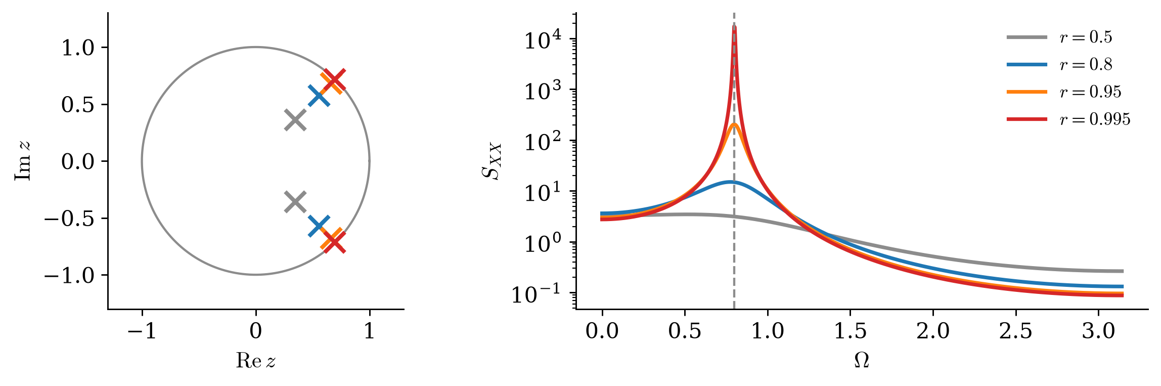
Figure 5: One conjugate pole pair of an AR(2) model, swept in radius: the angle sets where the spectral peak sits, the radius how sharp it is.

A pole near the unit circle is a spectral peak: the mechanism of a voiced-speech formant, two numbers per resonance.

AR(1): the one to keep in mind

\[X[k]=aX[k-1]+W[k],\qquad R_{XX}[\kappa]=\sigma_W^2\,\frac{a^{\abs\kappa}}{1-a^2},\qquad S_{XX}=\frac{\sigma_W^2}{\abs{1-ae^{-j\Omega}}^2} .\]

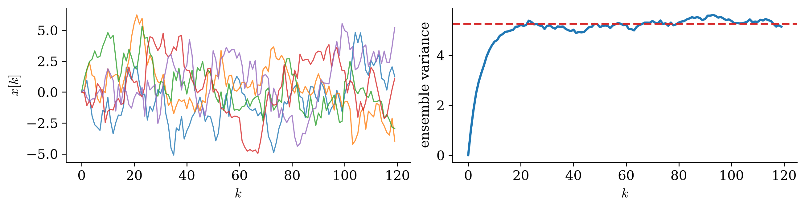
Figure 6: 3000 realizations of an AR(1) with a = 0.9, started from X[0] = 0: five paths, and the ensemble variance climbing to its stationary value.

Correlation decaying geometrically, and a start-up transient that a stable recursion forgets: a process can be non-stationary at the start and stationary and ergodic in the long run. Simulations discard a burn-in for this reason.

The residual is white

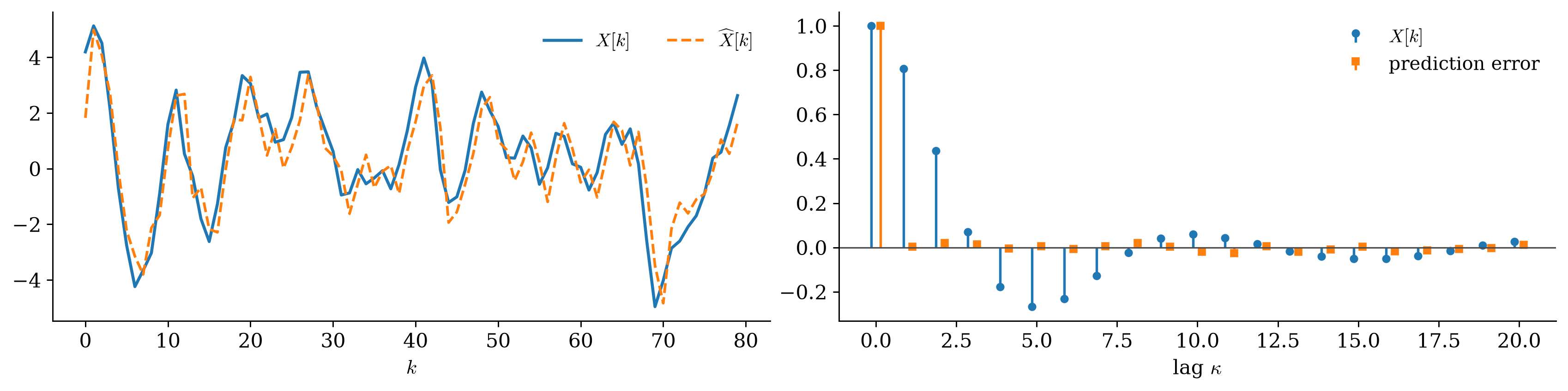
Figure 7: An AR(2) realization with its one-step prediction, and the autocorrelation before and after the prediction-error filter.

The signal is strongly correlated across lags; the residual is correlated with nothing. All the linear structure has moved into two coefficients.

Forecasting: the past loses its grip

For an AR(1) process, \(m\) steps ahead: \(\widehat X[k+m\mid k]=a^mX[k]\), with error variance \(\sigma_W^2\frac{1-a^{2m}}{1-a^2}\).

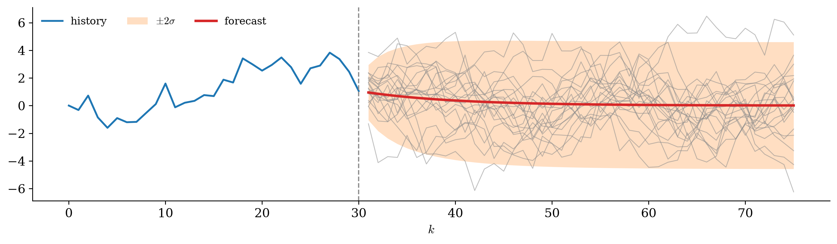
Figure 8: An AR(1) history, its forecast and ±2σ band, with twenty continuations.

The forecast relaxes to the mean and the band widens to the marginal spread: at long horizons prediction is no better than the unconditional mean.

What prediction buys: spectral flatness

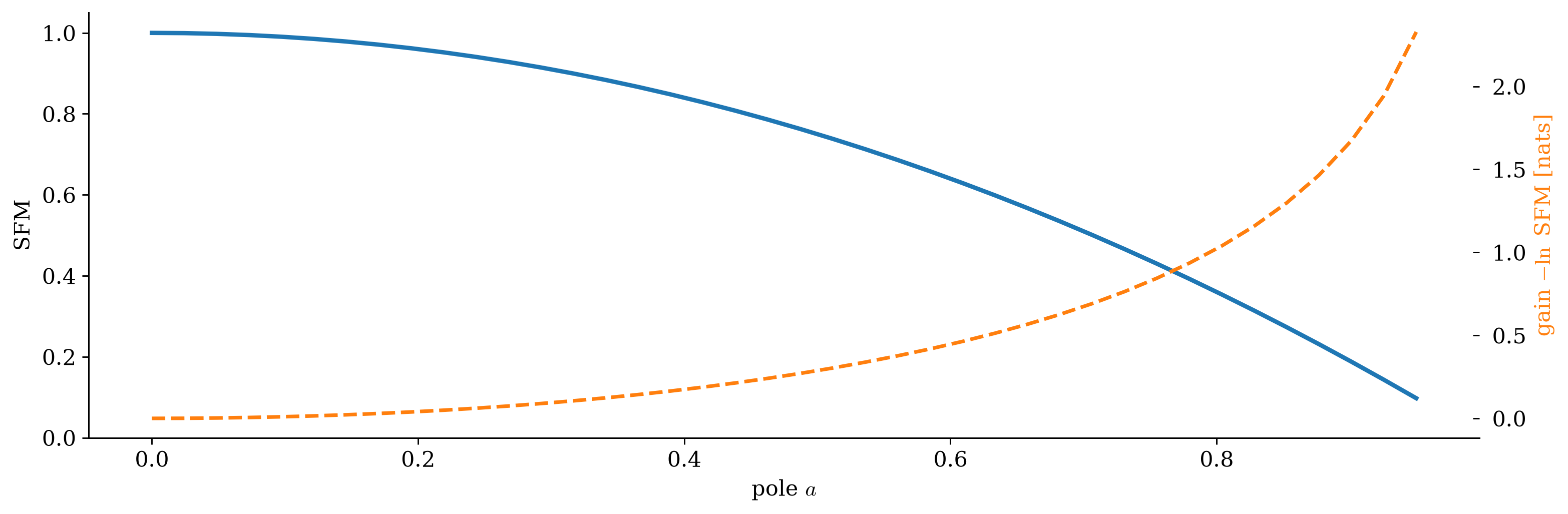
Spectral flatness \[\mathrm{SFM}=\frac{\exp\paren{\frac{1}{2\pi}\int\ln S_{XX}\dd\Omega}}{\frac{1}{2\pi}\int S_{XX}\dd\Omega} =\frac{\sigma_E^2}{\sigma_X^2}\in(0,1]:\] the geometric over the arithmetic mean of the spectrum.

What prediction buys: spectral flatness

Figure 9: Spectral flatness and prediction gain −ln SFM across AR(1) spectra with pole a.

A flat spectrum: no linear predictor beats zero. A peaky one: large prediction gain, which is also the ceiling on what a linear model can compress.

White is not unpredictable, again

The random-frequency tone of the stationary-process week has a flat spectrum, so \(\mathrm{SFM}=1\) and the best linear predictor gains nothing.

The random-frequency tone \(X[k+1]=2\cos(\Omega_0)X[k]-X[k-1]\): three samples identify the recurrence, and the best nonlinear prediction error is zero.

White means no second-order linear structure, not unpredictable, unless an extra assumption such as Gaussianity makes linear and nonlinear prediction coincide.

Linear predictive coding

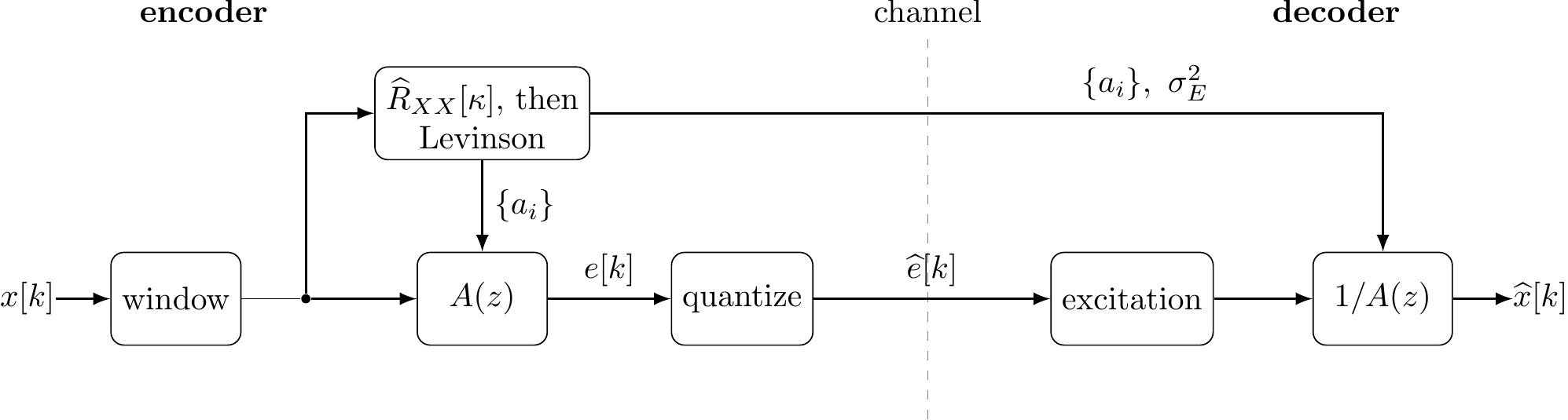
LPC: estimate the correlations of each window, solve Yule–Walker, send the coefficients and the residual; the decoder colors an excitation with \(1/A(z)\).

A resonant vowel has a peaky spectrum and predicts well; a hissing /s/ is nearly flat and does not. That is the whole reason LPC codecs handle vowels better than fricatives.

LPC on a real vowel

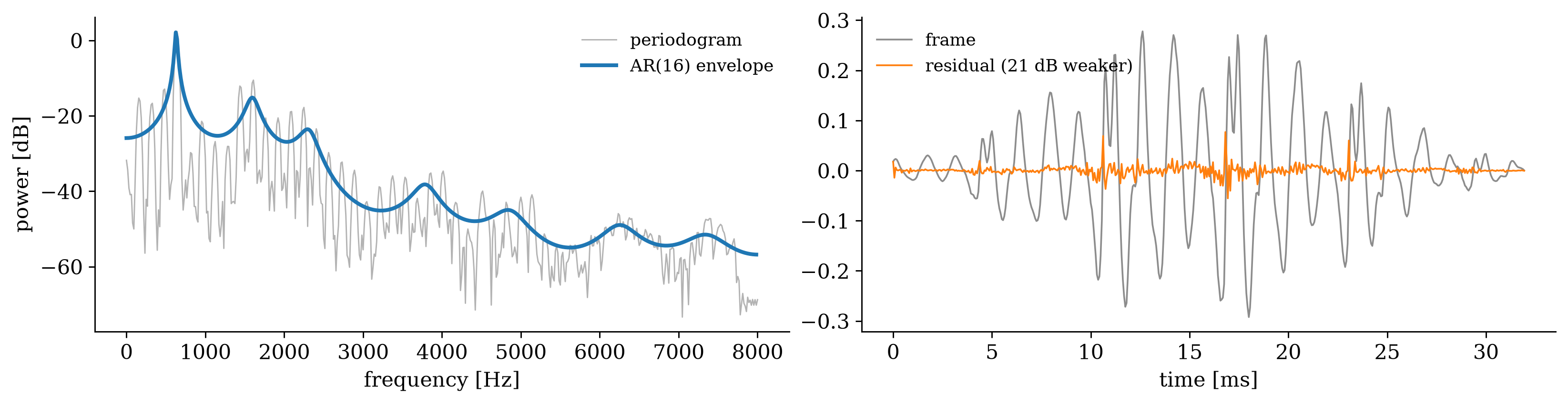
Figure 10: A 32 ms voiced frame of the speech recording: its periodogram and the order-16 AR (LPC) envelope from Yule–Walker (left), and the frame against its prediction residual (right).

Sixteen coefficients describe the formant envelope; what is left is a much weaker, nearly white residual with the pitch pulses in it. That residual is what an LPC coder spends its bits on.

Filtering and smoothing

Three tasks, three amounts of data

smoothing

filtering

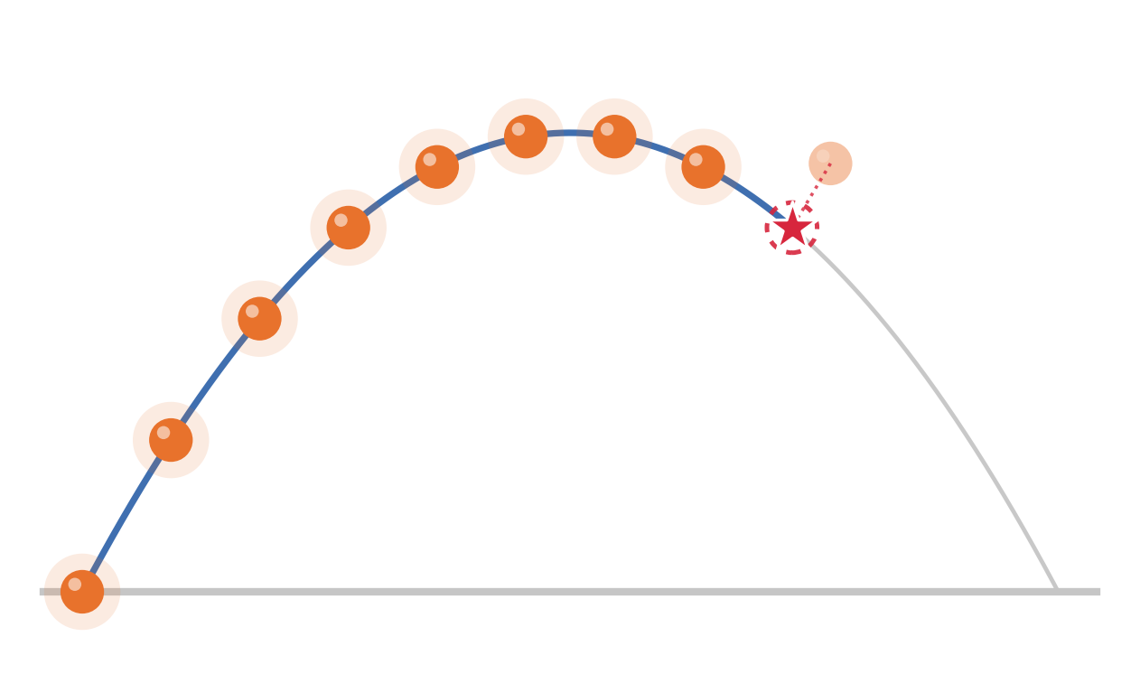
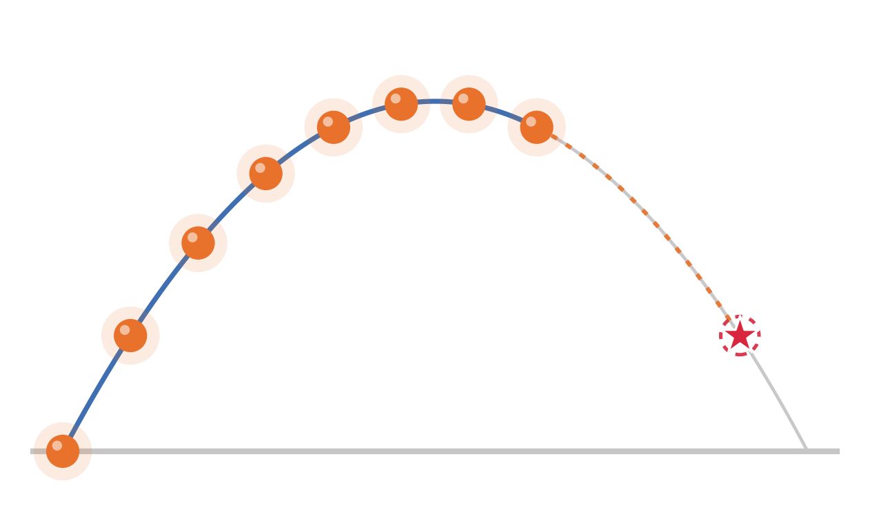
prediction

Data on both sides, the present and past, the past only: the subspace shrinks, so the error can only grow. Smoothing ≤ filtering ≤ prediction, one fact, not three.

Three tasks, three amounts of data

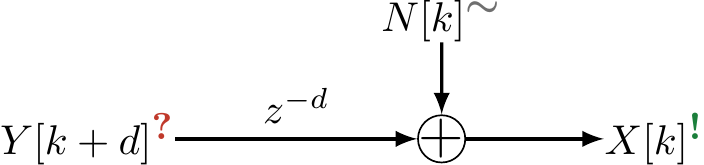
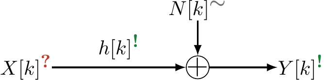
Estimation in noise as a signal flow. The sign of \(d\) names the task: \(d<0\) smoothing, \(d=0\) filtering, \(d>0\) prediction.

One Toeplitz matrix, a moving right-hand side

For a signal in white noise, \(X=Y+N\), with a window of \(L\) samples and the target \(d\) samples ahead of the window’s end:

Predict, filter, smooth \[\paren{\mathbf R_{\mathbf{YY}}+\sigma_N^2\mathbf I}\,\mathbf h\opt=\mathbf r_d,\qquad \mathbf r_d=\bracket{R_{YY}[d],\dots,R_{YY}[d+L-1]}\tran,\qquad \sigma_E^2=R_{YY}[0]-\mathbf r_d\herm\mathbf h\opt .\]

\(d>0\) predicts, \(d=0\) filters, \(d<0\) smooths. The matrix never changes; only which lags of the autocorrelation appear on the right.

A noisy track, three ways

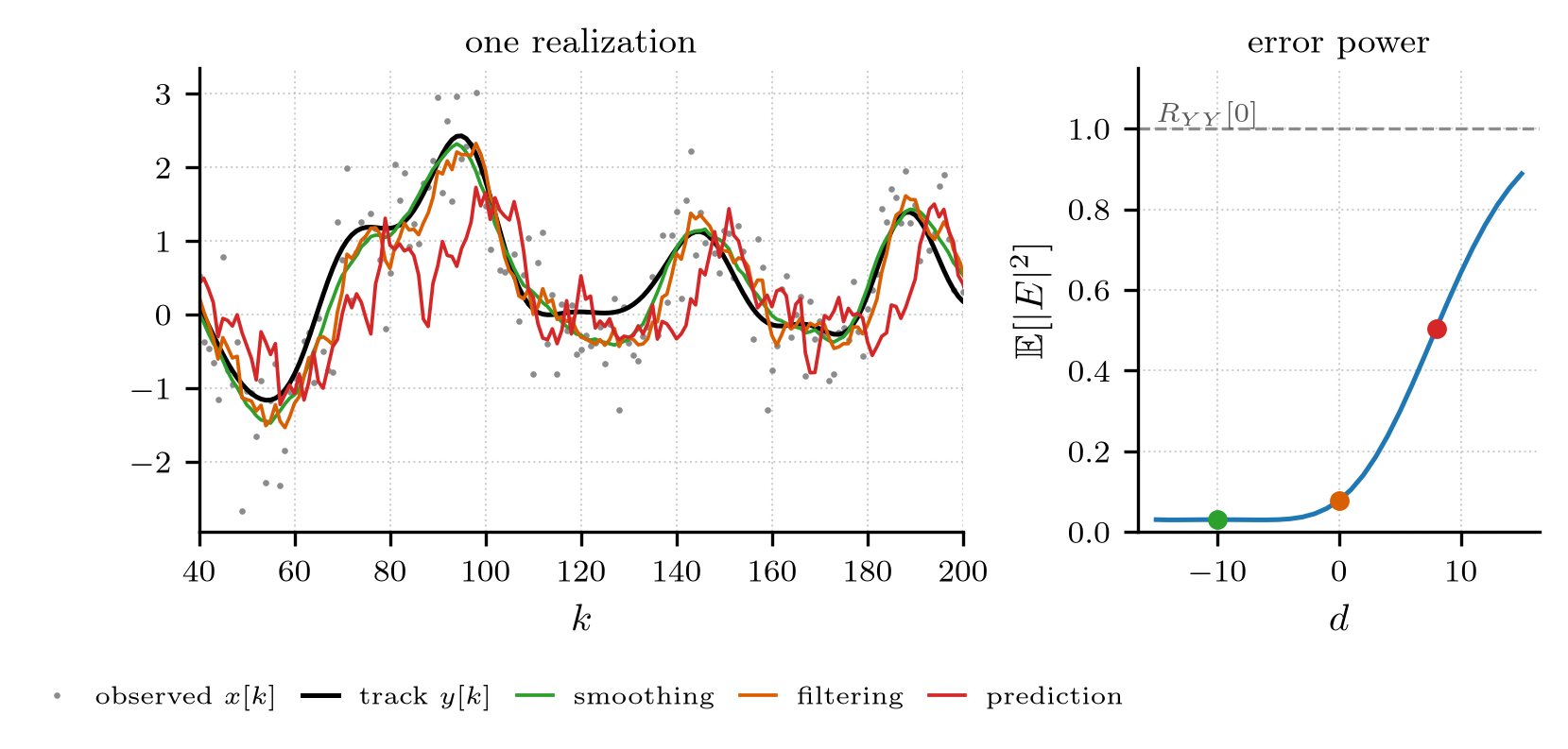
Left: a track, its noisy observation, and the predicted, filtered and smoothed estimates. Right: the error power against the position of the target inside the window.

The error is smallest for a target in the middle of the window, with data on both sides, and grows steeply once the target leaves it. Smoothing is cheapest when you can afford to wait.

→ Demo: smoothing, filtering and prediction

Deconvolution

The inverse problem, in frequency

A blur \(h\) and noise, in the letters of the inverse problem: \(Y=h*X+N\), the cause \(X\) sought. The Wiener–Hopf solution, with observation and target exchanged:

Wiener deconvolution \[H\opt=\frac{H\conj S_{XX}}{\abs{H}^2S_{XX}+S_{NN}}=\frac{H\conj}{\abs{H}^2+S_{NN}/S_{XX}} .\]

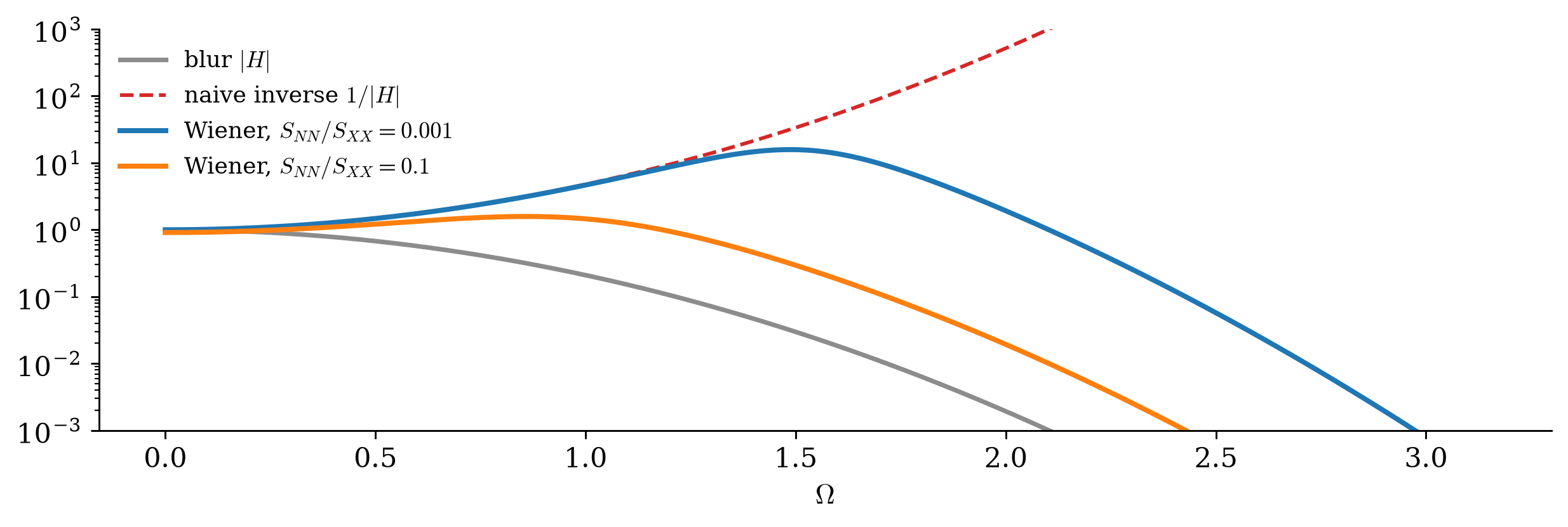
Where the blur passes signal, \(H\opt\approx1/H\): undo it. Where the blur kills a frequency, the noise-to-signal ratio stops the division from exploding.

The regularized inverse of the four-instruments week, diagonalized by the Fourier transform.

The inverse problem, in frequency

Deconvolution as a signal flow: the inverse problem of the four-instruments week, with the forward operator a filter.

The deconvolution gain

Figure 11: A Gaussian blur |H|, its naive inverse 1/|H|, and the Wiener deconvolution gain for two noise-to-signal ratios.

The Wiener gain follows the naive inverse while the blur still passes signal above the noise, then turns over and falls. The noisier the data, the earlier it gives up.

Deblurring an image

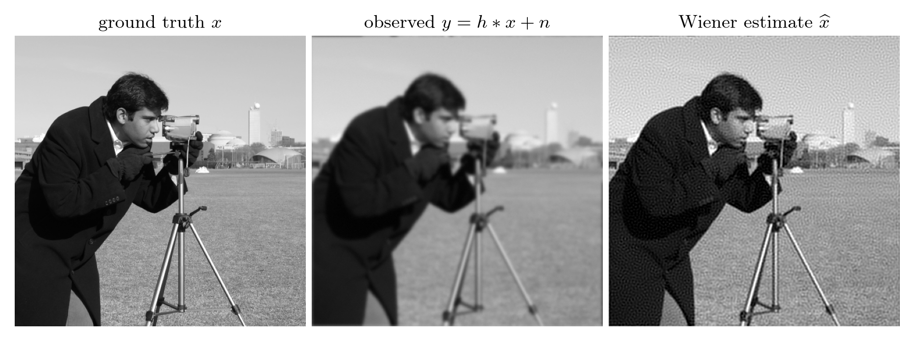
Ground truth, blurred and noisy observation, and the Wiener reconstruction.

Naive inversion would amplify noise wherever the blur suppressed the signal. The Wiener filter gives up exactly those frequencies, and the price is a little residual blur.

The matched filter, running

From inner product to convolution

With \(u\herm[k]=u\conj[-k]\) the adjoint sequence, the filter \(h=u\herm\) evaluated at the arrival reproduces the inner product exactly:

Matched filter as a convolution \[(u\herm*X)[k_0]=\sum_mX[m]\,u\conj[m-k_0]=\ip{\mathbf X,\mathbf u_{k_0}} .\]

In colored noise \(\mathbf R_{\mathbf{NN}}^{-1}\) becomes a division by the noise spectrum: \(H\opt\propto U\conj/S_{NN}\). Prewhiten, then correlate, frequency by frequency.

“Adjoint”, not “time reversal”: it keeps the conjugate for complex signals and survives on arrays, where there is no time axis to reverse.

A bank of detectors in one pass

One inner product tests one arrival time. Sliding the filter evaluates it at every candidate arrival at once, and the peak of the output locates the pulse.

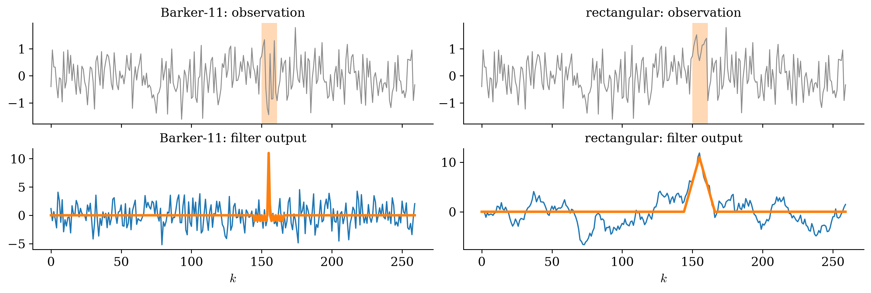
Top: an observation with a hidden Barker code. Bottom: the filter output, peaking at the arrival.

Detection and delay estimation are one computation: the same device measures range in radar and recovers symbol timing in a receiver.

A bank of detectors in one pass

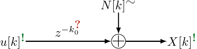
The running matched filter as a signal flow: the template known, the question mark on its delay.

Energy detects, the autocorrelation locates

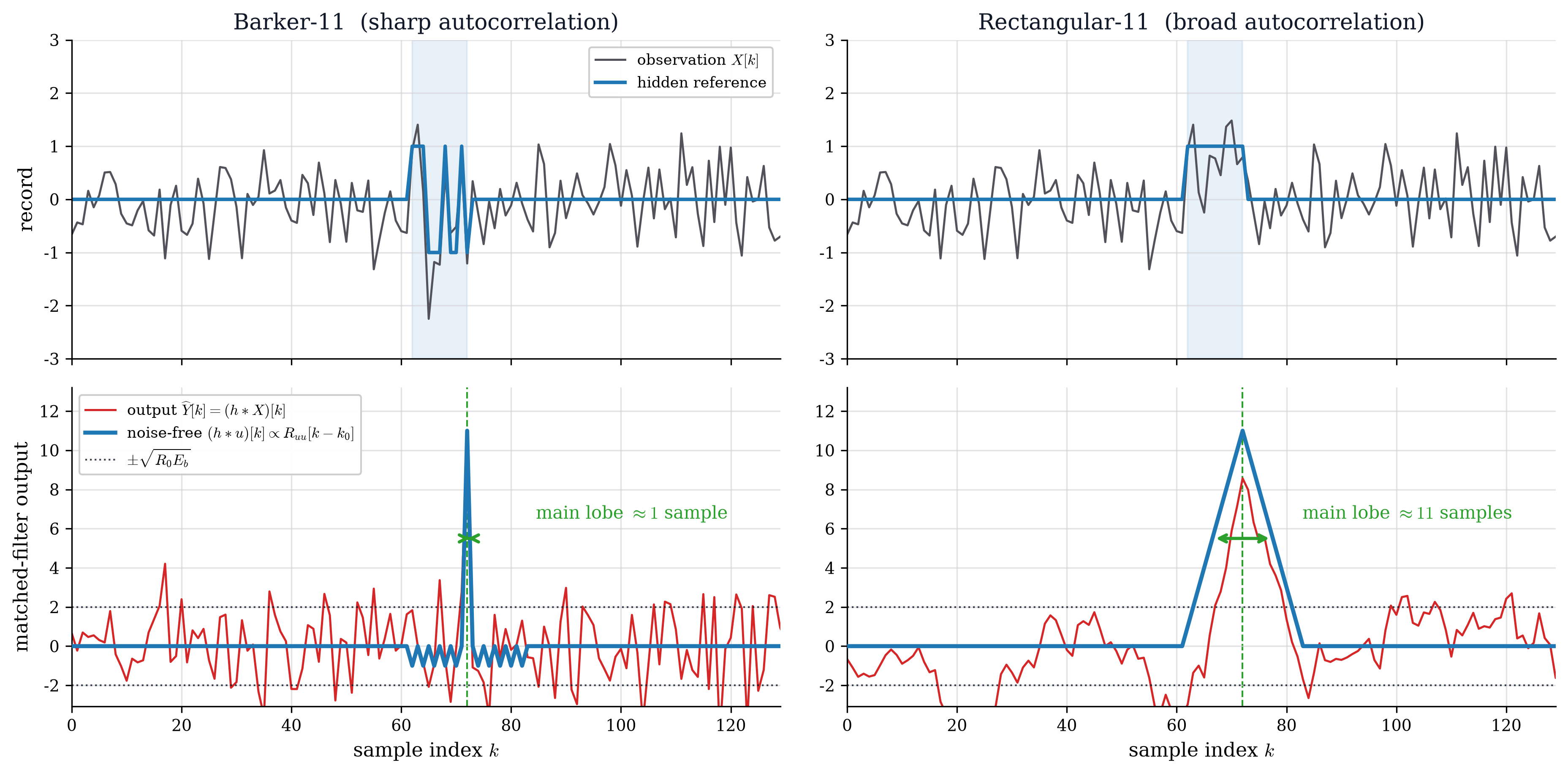
In noise-free terms the output is the template’s own autocorrelation, \(R_{uu}[k-k_0]\), centered on the arrival.

Two questions, two properties

• Detection cares only about the peak, the energy \(E_u\), whatever the shape.
• Delay estimation cares about how sharp the peak is: entirely a matter of shape.

A Barker code or chirp has the energy of a long pulse and the autocorrelation of a short one: that is why radars transmit coded pulses.

Same energy, different resolution

Figure 12: A Barker-11 code and a rectangular pulse of equal length and energy, hidden at the same instant in the same noise; orange is the noise-free output.

Both outputs peak at the same height, the energy 11: equally detectable. The Barker output is one sample wide, the rectangular one eleven.

Broadband sources localize well

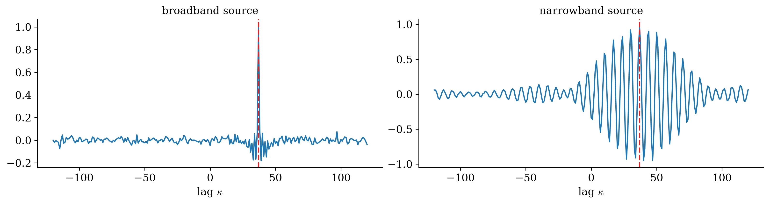
Figure 13: Two recordings of one source, offset by 37 samples and independently noisy: the cross-correlation for a broadband and a narrowband source.

A narrowband source is correlated with itself at every period, so its cross-correlation has many nearly equal peaks and the delay becomes ambiguous. Perfect predictability and perfect localization are opposites.

Coherence: what a linear filter can explain

Coherence \[\abs{\rho_{YX}}^2=\frac{\abs{S_{YX}}^2}{S_{XX}S_{YY}},\qquad S_{EE}=S_{YY}\paren{1-\abs{\rho_{YX}}^2}.\]

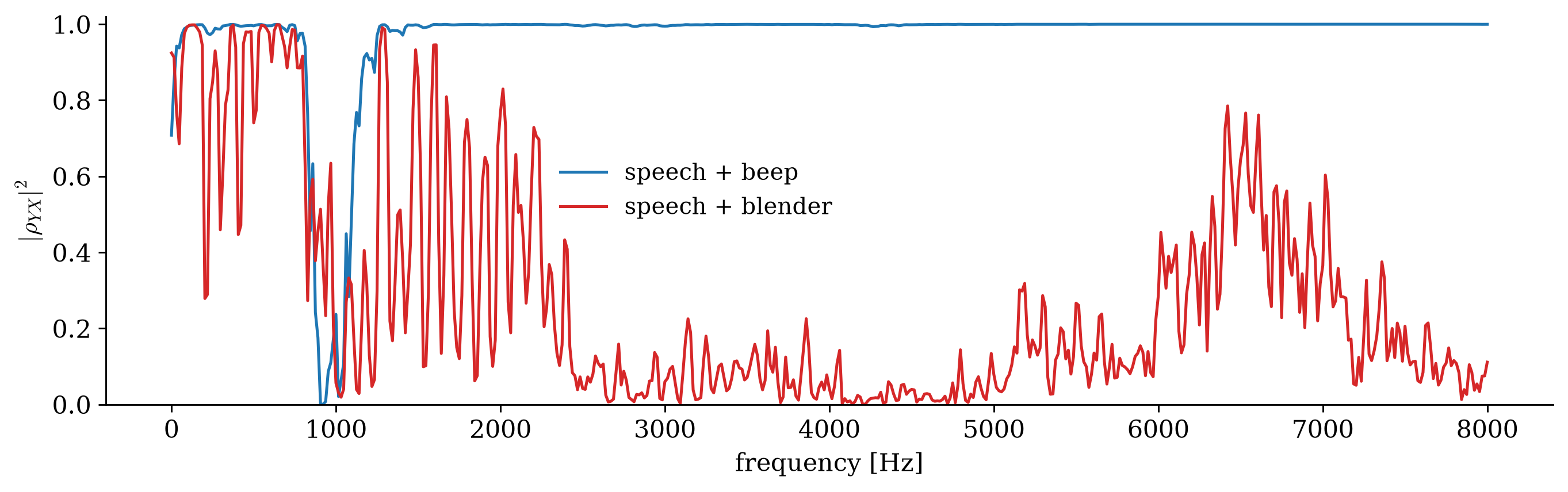
Coherence one: the target is a linear function of the observation there, recovered exactly. Coherence zero: nothing linear can help.

The correlation coefficient of the random-vector week, frequency by frequency, known before designing anything.

Coherence, measured

Figure 14: Magnitude-squared coherence between the clean speech and each noisy recording, estimated by averaging over 1024-sample segments.

The beep drops the coherence only in a few narrow bands; the blender drops it almost everywhere. The two SNR gains of the denoising demo, \(+22.5\) and \(+3.5\) dB, were visible here before any filter was built.

Broadband arrays

Why space alone stops being enough

A narrowband delay is one phase per sensor, so one complex weight per sensor steers the array. A broadband delay is a different phase at every frequency: each channel needs its own filter.

Space–time snapshot Stack the last \(L\) snapshots of \(M\) sensors: \[\underline{\mathbf X}[k]=\bracket{\mathbf X[k]\tran,\dots,\mathbf X[k-L+1]\tran}\tran\in\Complex^{ML},\qquad \widehat Y[k]=\underline{\mathbf w}\herm\underline{\mathbf X}[k].\]

MMSE and MVDR return unchanged, with a block-Toeplitz correlation matrix. No new theory, a longer vector.

A delay is a phase ramp

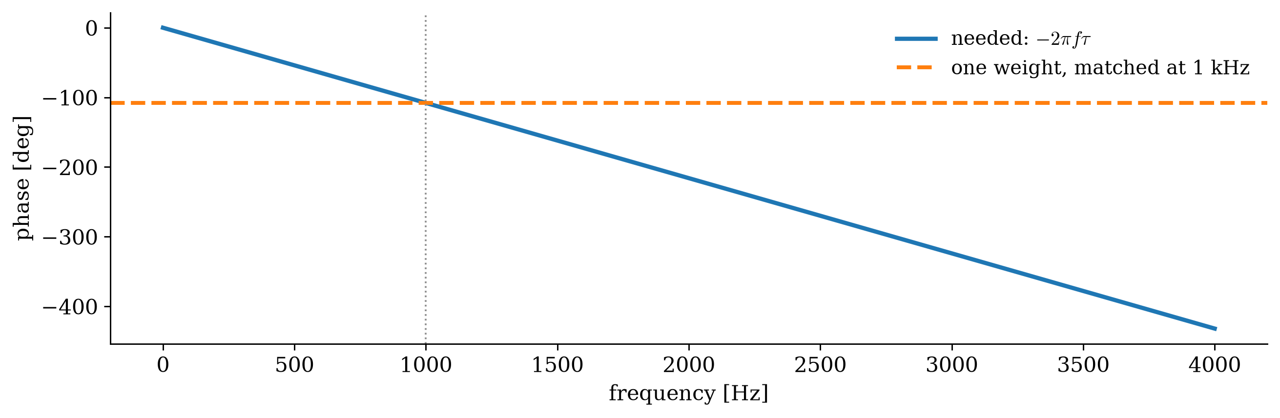
Figure 15: The phase a delay of τ = 0.3 ms imposes at each frequency (blue), and the phase a single complex weight provides (orange), tuned at 1 kHz.

A narrowband weight matches the delay at one frequency and is wrong everywhere else. Matching a ramp needs a filter per sensor: a fractional delay, which is what the space–time vector provides.

A real array, a real scene

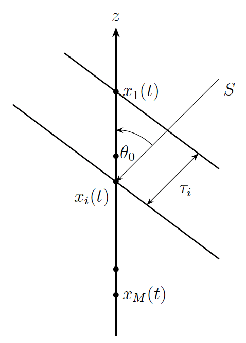
A line array: a source at angle \(\theta_0\) reaches each microphone with its own delay.

 

A talker at 90°, a blender at 120°, rustling paper at 45°. One microphone, everything jumbled together:

The MVDR output, one weight vector per frequency, told only where the talker is:

Where the nulls went

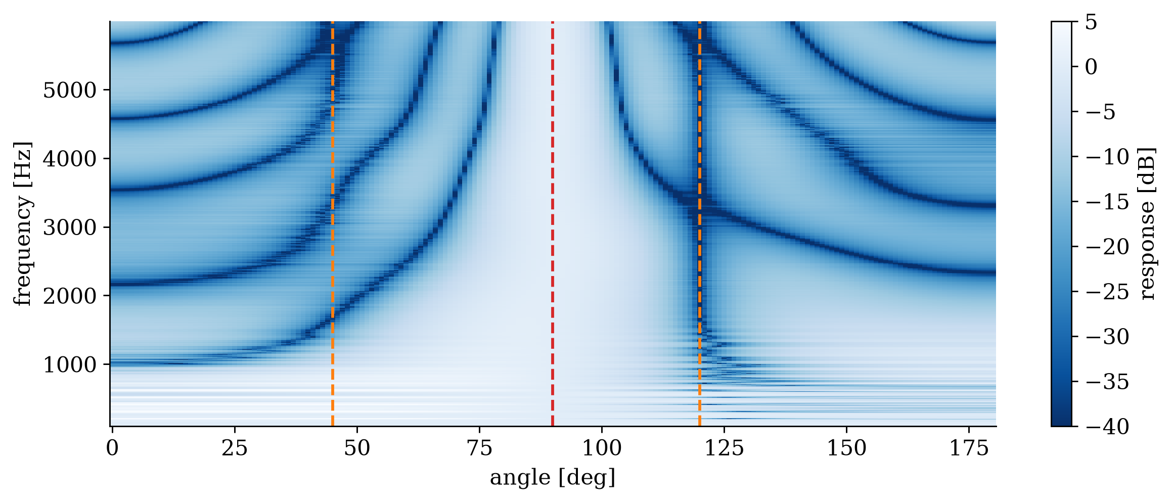
Figure 16: The MVDR spatial response against frequency: unit gain toward the talker (red) at every frequency, nulls following the two interferers (orange).

Each frequency sees the same geometry differently, so each gets its own weights. Below about 1 kHz the array is small against the wavelength and can barely steer; above \(c/2d\approx3.4\) kHz the spacing violates half a wavelength and grating lobes appear.

Recap

This week

1. Orthogonality on a process gives the Wiener–Hopf equation: the normal equations as a convolution, and in frequency one ratio \(S_{YX}/S_{XX}\) per frequency. Denoising passes each frequency in proportion to its share of signal.

2. The same Toeplitz system answers many questions: system identification (white input: correlation is the answer), prediction (Yule–Walker; its error is white; flatness is its gain), filtering and smoothing (only the right-hand side moves), deconvolution.

3. The matched filter and the beamformer run in time too. Energy sets detectability, the autocorrelation sets resolution, and a broadband array is the vector problem on a space–time vector, solved one frequency at a time.