Physical and numerical parameters:
  String length L = 1.0 m
  Wave speed c = 300.0 m/s
  Number of interior grid points M = 80
  Spatial step h = 0.012346 m
  Sample rate fs = 44100.0 Hz
  Time step T = 0.00002268 s
Courant number λ = 0.5510201 Functional Transformation Methods from a Discrete-Time View
In this notebook, we study an example of the transverse waves of a thin string using the functional transformation method, proceeding from finite difference time domain (FDTD) discretization through Z-transform analysis to eigenvalue decomposition (EVD).
Listen to sound demos of the physical string modeling made by Ableton’s Tension.
For a numerical example, let’s assume the following physical parameters.
1.1 Continuous-time string model
Consider a thin, perfectly flexible string of length L with transverse displacement y(x,t), wave speed c, and external excitation v(x,t).
The PDE is the (driven) 1D wave equation c^{-2}\,\frac{\partial^2 y(x,t)}{\partial t^2} - \frac{\partial^2 y(x,t)}{\partial x^2} = v(x,t), \qquad 0 < x < L,\; t > 0.
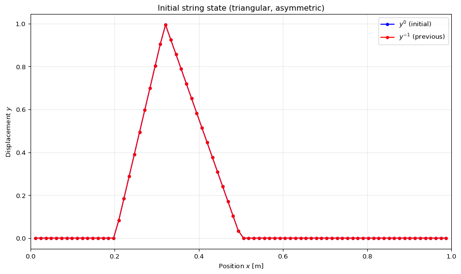
Initial conditions are encoded by an operator f_i as f_i\{y(x,0)\} = \mathbf y_i(x) = \begin{bmatrix} y_{i0}(x)\\[2pt] y_{i1}(x) \end{bmatrix} = \begin{bmatrix} y(x,0)\\[2pt] \dot y(x,0) \end{bmatrix}.
For a string fixed at both ends (Dirichlet boundaries) y(0,t) = 0, \qquad y(L,t) = 0.
For the FDTD example below, we will set v(x,t)=0 (excitation only via initial conditions).
1.2 FDTD discretization of the wave equation
1.2.1 Space and time grids
Let
- h be the spatial step,
- T be the time step,
- x_m = m\,h,\quad m = 0,\dots,M+1,\quad L = (M+1)h,
- t^k = k\,T,\quad k = 0,1,2,\dots
We approximate y_m^k \approx y(x_m,t^k).
The interior grid points are m = 1,\dots,M; the boundary points m=0 and m=M+1 are fixed to zero.
Define the Courant number \lambda = \frac{c\,T}{h}.
1.2.2 Finite differences
Second-order central differences:
Time: \frac{\partial^2 y}{\partial t^2}(x_m,t^k) \approx \frac{y_m^{k+1} - 2 y_m^k + y_m^{k-1}}{T^2}.
Space: \frac{\partial^2 y}{\partial x^2}(x_m,t^k) \approx \frac{y_{m+1}^k - 2 y_m^k + y_{m-1}^k}{h^2}.
Inserting into the PDE with v(x,t)=0 gives c^{-2} \frac{y_m^{k+1} - 2 y_m^k + y_m^{k-1}}{T^2} - \frac{y_{m+1}^k - 2 y_m^k + y_{m-1}^k}{h^2} = 0.
Multiplying by c^2 T^2 and noting that from the Courant number definition \lambda = c T / h we have \lambda^2 = c^2 T^2 / h^2:
y_m^{k+1} - 2 y_m^k + y_m^{k-1} - \lambda^2 \left( y_{m+1}^k - 2 y_m^k + y_{m-1}^k \right) = 0.
Solving for y_m^{k+1} gives the explicit update y_m^{k+1} = 2 (1-\lambda^2)\,y_m^k + \lambda^2 (y_{m+1}^k + y_{m-1}^k) - y_m^{k-1}, \qquad m=1,\dots,M.
Boundary conditions: y_0^k = 0,\qquad y_{M+1}^k = 0,\quad \forall k.
Stability of this explicit scheme requires \lambda \le 1.
1.3 Matrix form of the spatial operator
Define the vector of interior points \mathbf y^k = \begin{bmatrix} y_1^k\\ y_2^k\\ \vdots\\ y_M^k \end{bmatrix} \in\mathbb R^M.
Introduce the discrete Laplacian matrix (Dirichlet boundaries) \mathbf L = \begin{bmatrix} -2 & 1 & 0 & \cdots & 0\\ 1 & -2 & 1 & \ddots & \vdots\\ 0 & 1 & -2 & \ddots & 0\\ \vdots & \ddots & \ddots & \ddots & 1\\ 0 & \cdots & 0 & 1 & -2 \end{bmatrix} \in \mathbb R^{M\times M}.
Then, for interior points, \frac{\partial^2 y}{\partial x^2}(x_m,t^k) \;\Rightarrow\; \frac{1}{h^2}\,(\mathbf L\mathbf y^k)_m.
The discrete update for the whole vector becomes (using the Courant number \lambda = c T / h defined above) \mathbf y^{k+1} = \left(2\mathbf I + \lambda^2 \mathbf L \right)\mathbf y^k - \mathbf y^{k-1}, with \mathbf I the M\times M identity matrix.
This is a second-order (in time) vector difference equation.
1.4 First-order state-space formulation
To connect with standard digital filter / Z-transform notation, rewrite the scheme as a first-order state-space model.
Define the state vector \mathbf{\underline{y}}^k = \begin{bmatrix} \mathbf y^k\\[2pt] \mathbf y^{k-1} \end{bmatrix} \in\mathbb R^{2M}.
Then \begin{aligned} \mathbf y^{k+1} &= \left(2\mathbf I + \lambda^2 \mathbf L \right)\mathbf y^k - \mathbf y^{k-1},\\ \mathbf y^{k} &= 1\cdot \mathbf y^{k} + 0\cdot \mathbf y^{k-1}. \end{aligned}
Thus, \mathbf{\underline{y}}^{k+1} = \mathbf A\,\mathbf{\underline{y}}^k, with \mathbf A = \begin{bmatrix} 2\mathbf I + \lambda^2 \mathbf L & -\mathbf I\\[4pt] \mathbf I & \mathbf 0 \end{bmatrix} \in\mathbb R^{2M\times 2M}, and \mathbf 0 the M\times M zero matrix.
Initial state \mathbf{\underline{y}}^0 is determined from the continuous initial conditions \mathbf y^0 = \mathbf y_i(x)\ \text{sampled},\qquad \mathbf y^{-1} \approx \mathbf y^0 - T\,\mathbf y_{i1}(x)\ \text{sampled}, i.e. by a backward Euler step for the initial velocity.
At this point we have a purely discrete-time, finite-dimensional LTI system. The connection to FTM comes from:
- Z-transform in time,
- Diagonalisation of the spatial operator (or of \mathbf A).
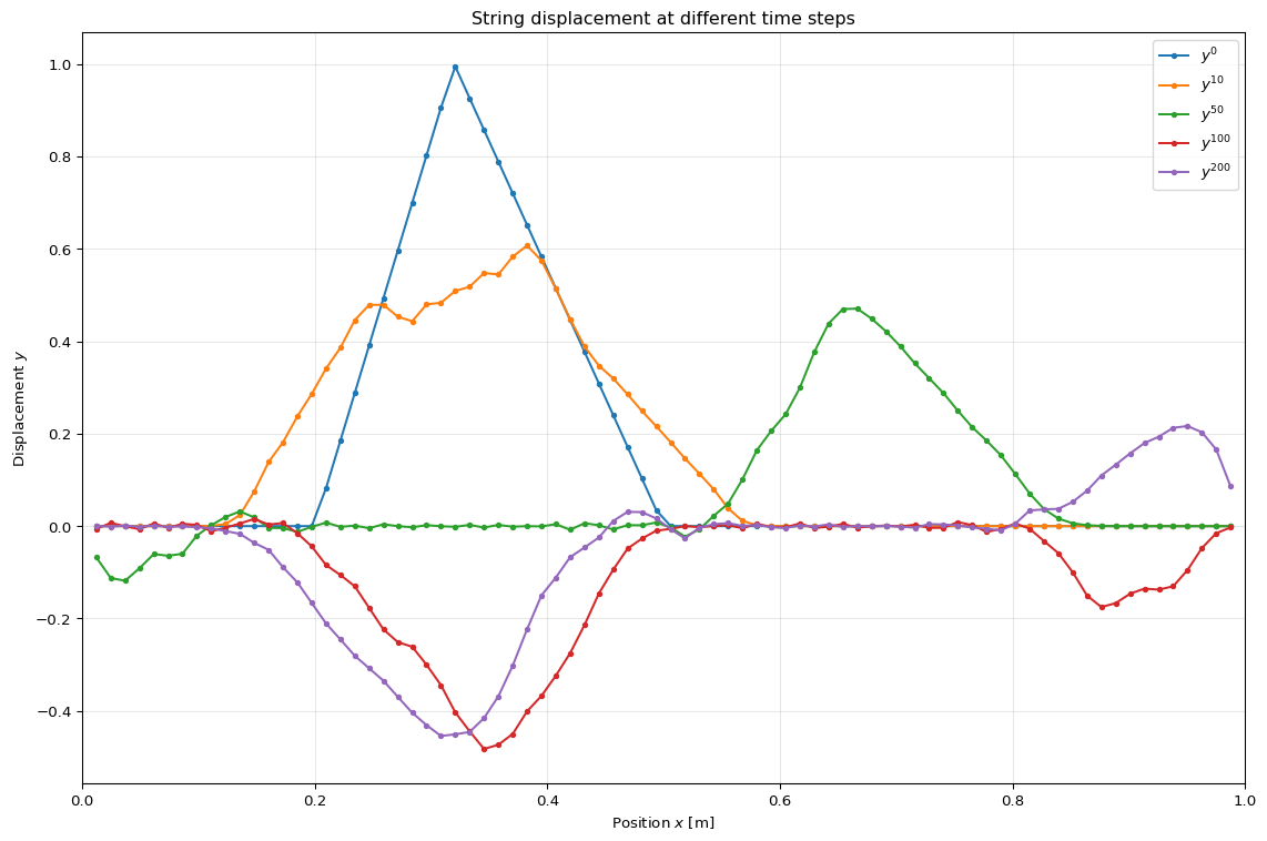
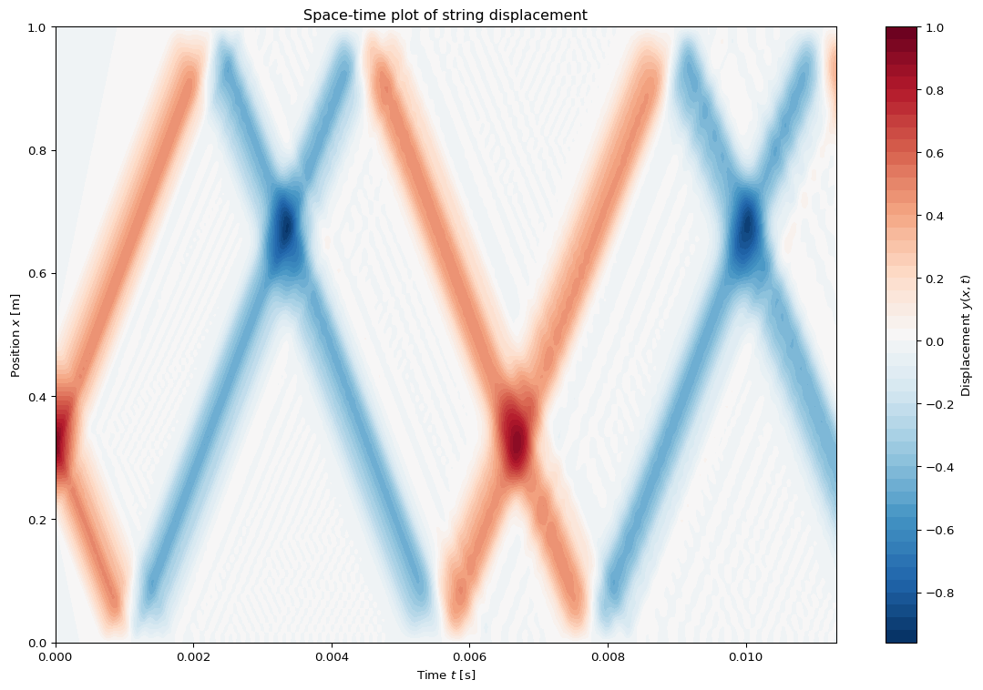
The animation below shows the string displacement evolving over time:
1.5 Z-transform in time
Apply the unilateral Z-transform to the state equation \mathbf{\underline{y}}^{k+1} = \mathbf A\,\mathbf{\underline{y}}^k, \qquad k\ge 0.
With \mathbf{\underline{Y}}(z) = \sum_{k=0}^\infty \mathbf{\underline{y}}^k z^{-k}, and using the standard shift property \mathcal Z\{\mathbf{\underline{y}}^{k+1}\} = z\mathbf{\underline{Y}}(z) - z\mathbf{\underline{y}}^0, we obtain z\mathbf{\underline{Y}}(z) - z\mathbf{\underline{y}}^0 = \mathbf A\,\mathbf{\underline{Y}}(z).
Rearranging: (z\mathbf I_{2M} - \mathbf A)\,\mathbf{\underline{Y}}(z) = z\,\mathbf{\underline{y}}^0.
Thus the Z-domain solution is \mathbf{\underline{Y}}(z) = (z\mathbf I_{2M} - \mathbf A)^{-1} z\,\mathbf{\underline{y}}^0.
This is the direct discrete-time analogue of the Laplace-domain solution \mathbf{\underline{Y}}(s) = (s\mathbf I - \mathbf A_c)^{-1} \mathbf{\underline{y}}(0) for continuous-time state-space systems.
The poles of the string model are the eigenvalues of \mathbf A, i.e. the roots of \det(z\mathbf I_{2M} - \mathbf A) = 0.
However, instead of diagonalising the full 2M \times 2M matrix \mathbf A, it is more transparent to diagonalise the spatial Laplacian \mathbf L first.
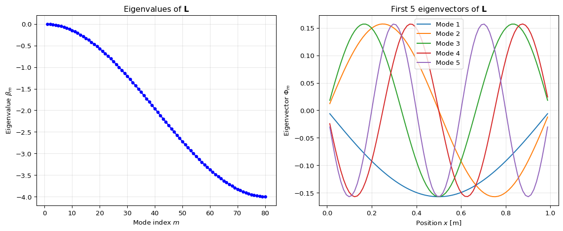
1.6 Spatial eigen-decomposition (discrete Sturm–Liouville step)
The matrix \mathbf L is real symmetric and tridiagonal, so it admits an eigenvalue decomposition \mathbf L = \mathbf\Phi\,\mathbf\Lambda\,\mathbf\Phi^\top, with
- \mathbf\Phi \in \mathbb R^{M\times M} orthogonal (\mathbf\Phi^\top\mathbf\Phi=\mathbf I),
- \mathbf\Lambda = \operatorname{diag}(\mu_1,\dots,\mu_M) containing the eigenvalues.
For the Dirichlet string the eigenvectors and eigenvalues are known analytically:
Eigenvectors (discrete sines) \Phi_{m_1 m_2} = \sqrt{\frac{2}{M+1}}\, \sin\left(\frac{\pi m_2 m_1}{M+1}\right), \quad m_1,m_2 = 1,\dots,M.
Eigenvalues \beta_m = -4\,\sin^2\!\left(\frac{\pi m}{2(M+1)}\right),\qquad m = 1,\dots,M.
Define the modal coordinates \boldsymbol\eta^k = \mathbf\Phi^\top \mathbf y^k.
Insert \mathbf y^k = \mathbf\Phi \boldsymbol\eta^k into the second-order vector update: \begin{aligned} \mathbf\Phi \boldsymbol\eta^{k+1} &= \left(2\mathbf I + \lambda^2 \mathbf L \right)\mathbf\Phi \boldsymbol\eta^k - \mathbf\Phi \boldsymbol\eta^{k-1} \\[4pt] &= \left(2\mathbf I + \lambda^2 \mathbf\Phi\mathbf\Lambda\mathbf\Phi^\top\right)\mathbf\Phi \boldsymbol\eta^k - \mathbf\Phi \boldsymbol\eta^{k-1}. \end{aligned}
Using \mathbf\Phi^\top\mathbf\Phi=\mathbf I and left-multiplying by \mathbf\Phi^\top: \boldsymbol\eta^{k+1} = \left(2\mathbf I + \lambda^2 \mathbf\Lambda\right)\boldsymbol\eta^k - \boldsymbol\eta^{k-1}.
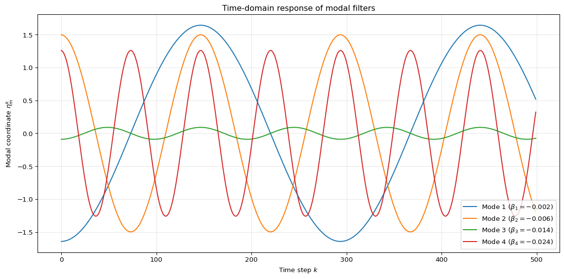
This is now diagonal in mode index \mu. For each mode \mu: \eta_{\mu}^{k+1} = \alpha_{\mu} \,\eta_{\mu}^k - \eta_{\mu}^{k-1}, \qquad \alpha_{\mu} = 2 + \lambda^2 \beta_{\mu}.
Thus the full string model is a parallel bank of independent second-order IIR sections, one per mode.
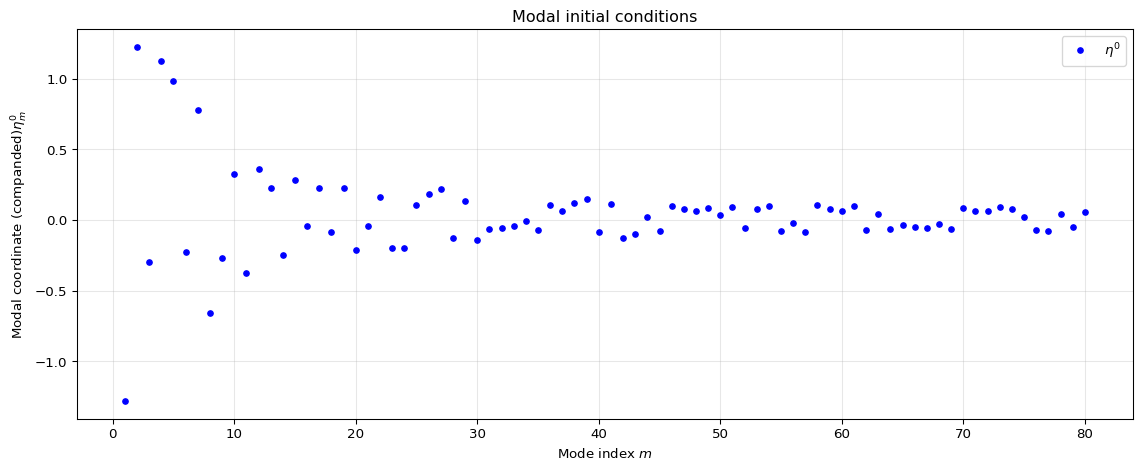
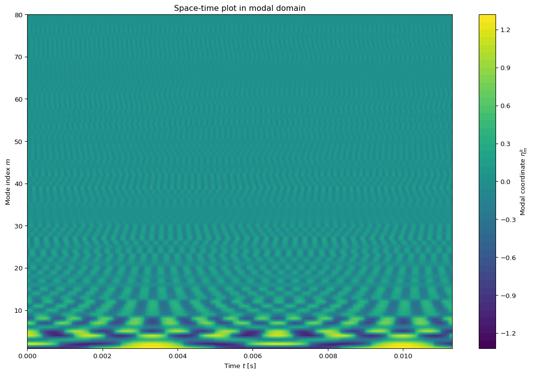
For better visualization, the amplitude of the modal coordinate is companded by
\mathrm{companded(\eta_m^k)} = \mathrm{sign}(\eta_m^k) \sqrt{|\eta_m^k|}
The modal coordinates evolve over time according to their second-order dynamics: 
The modal-temporal dynamics are plotted as a 2D plot below.
1.7 Z-transform of each mode (discrete modal filters)
Taking the unilateral Z-transform of a single mode: \eta_{\mu}^{k+1} = \alpha_{\mu} \eta_{\mu}^k - \eta_{\mu}^{k-1} gives \begin{aligned} z\Eta_{\mu}(z) - z\eta_{\mu}^0 &= \alpha_{\mu} \left(\Eta_{\mu}(z) - \eta_{\mu}^0\right) - \left(z^{-1}\Eta_{\mu}(z) - z^{-1}\eta_{\mu}^0\right), \end{aligned} where \Eta_{\mu}(z) is the Z-transform of \eta_{\mu}^k.
Rearranging terms in \Eta_{\mu}(z) yields \left(z^2 - \alpha_{\mu} z + 1\right) \Eta_{\mu}(z) = \left(z^2 - \alpha_{\mu} z + 1\right)\eta_{\mu}^0 + (z-1) z\,\eta_{\mu}^1, where the exact right-hand side depends on how initial conditions are encoded. The characteristic polynomial is p_{\mu}(z) = z^2 - \alpha_{\mu} z + 1.
The two poles of mode \mu are z_{\mu,\pm} = \frac{\alpha_{\mu}}{2} \pm \sqrt{\left(\frac{\alpha_{\mu}}{2}\right)^2 - 1}.
For a stable string scheme with \lambda \le 1, the poles lie on (or close to) the unit circle and can be written (approximately) as z_{\mu,\pm} \approx e^{\pm \mathrm j \Omega_{\mu}}, where the discrete-time modal frequency \Omega_{\mu} satisfies \cos \Omega_{\mu} = \frac{\alpha_{\mu}}{2} = 1 + \frac{\lambda^2}{2} \beta_{\mu}.
Using the analytical \beta_{\mu} above gives the familiar modal frequencies of the discrete string.
Thus the complete procedure
- FDTD discretization \Rightarrow vector difference equation,
- Z-transform in time \Rightarrow algebraic equation in z with spatial operator \mathbf L,
- Eigen-decomposition of \mathbf L (discrete Sturm–Liouville) \Rightarrow independent 2nd-order sections,
is the exact discrete-time analogue of the continuous FTM with Laplace transform plus Sturm–Liouville eigen-expansion.
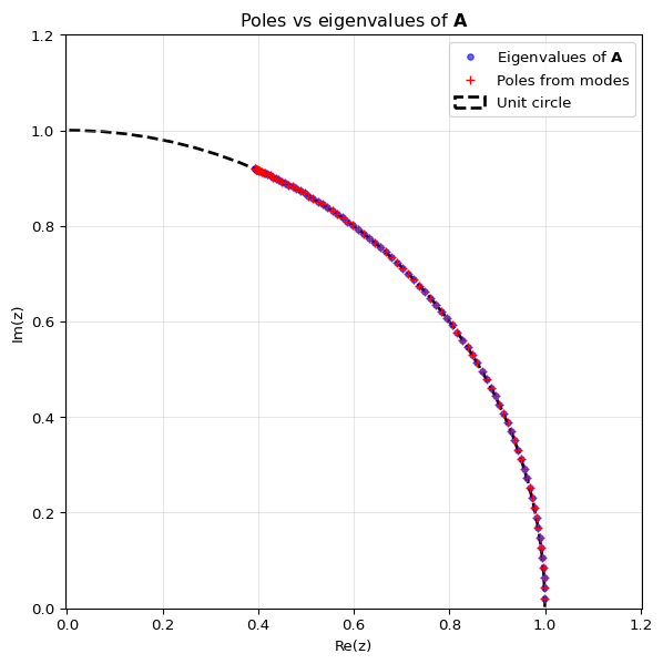
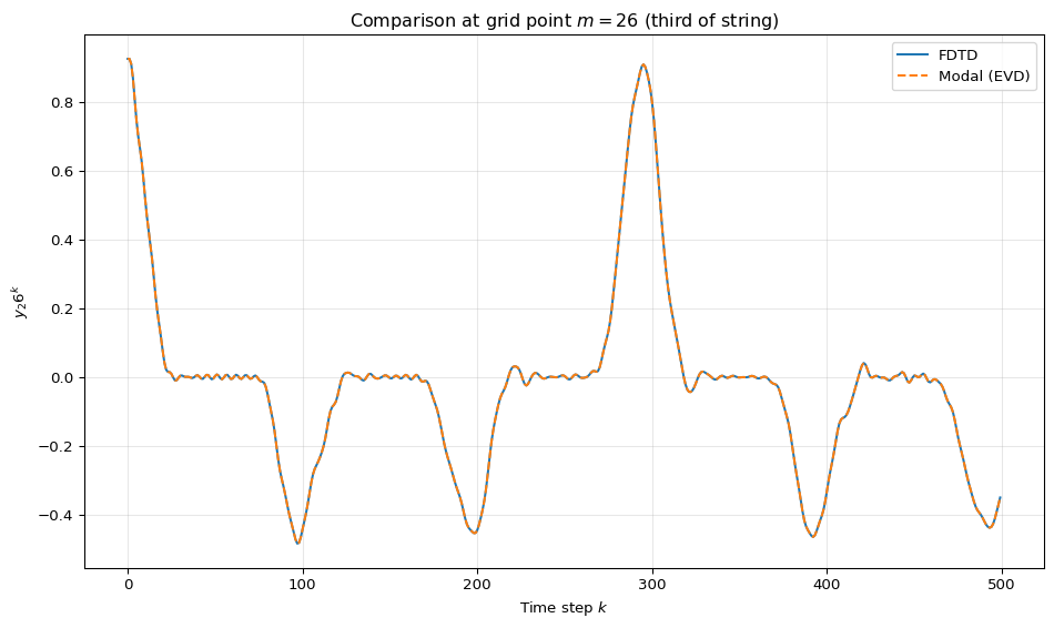
The two curves should coincide up to numerical precision, illustrating that
- FDTD in the physical domain, and
- modal IIR sections obtained via Z-transform + eigen-decomposition,
represent the same discrete-time system.
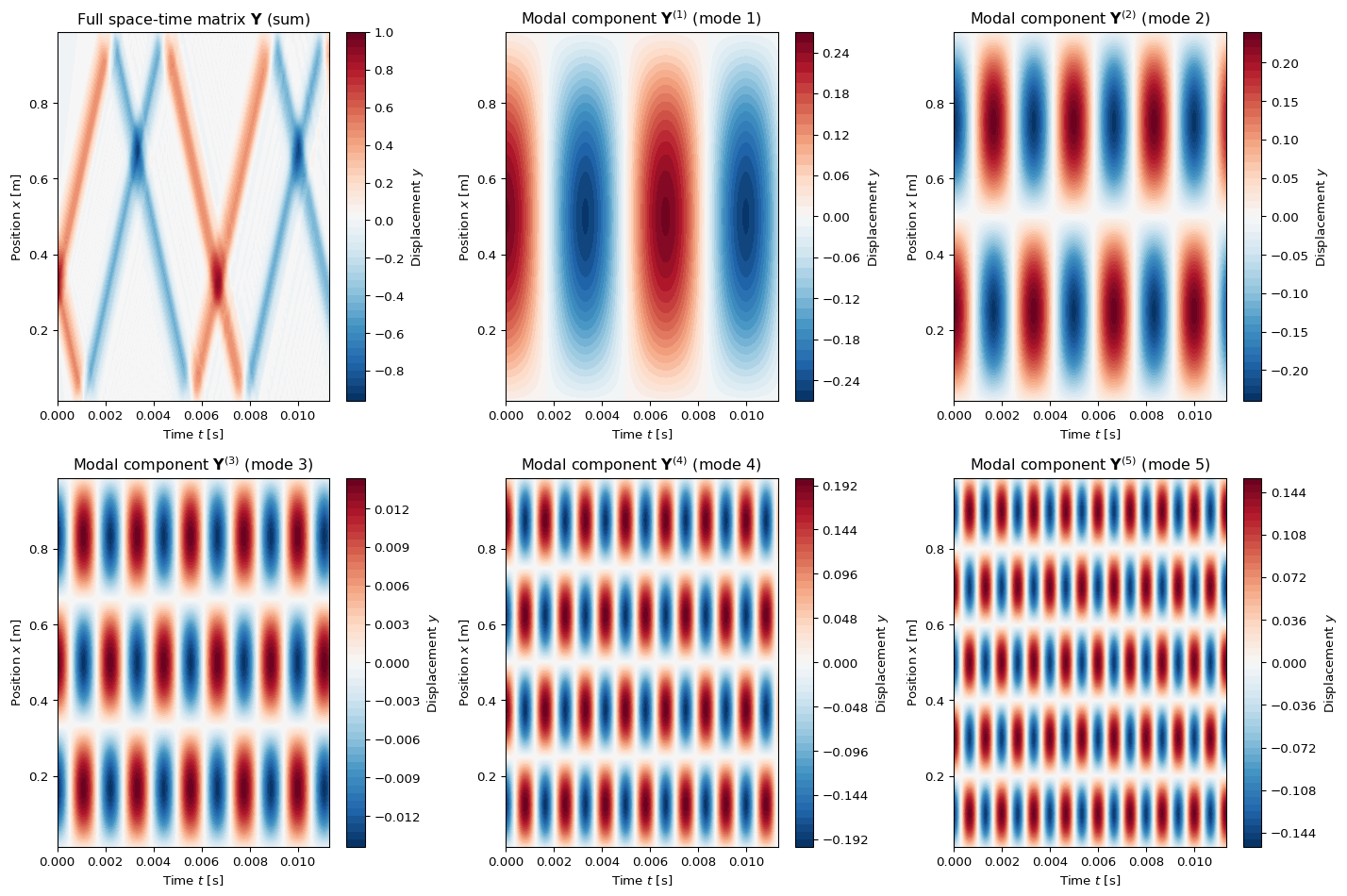
1.8 Modal view of the space-time separability
The space-time matrix \mathbf Y with entries Y_{k,m} = y_m^k (displacement at spatial point m and time step k) can be decomposed in terms of modal coordinates.
Using the modal decomposition \mathbf y^k = \mathbf\Phi \boldsymbol\eta^k, the space-time matrix can be written as a sum over modes:
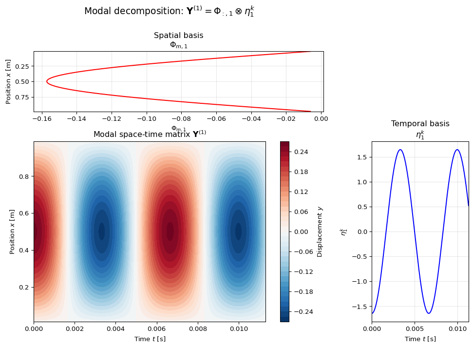
\mathbf Y = \sum_{\mu=1}^{M} \mathbf Y^{(\mu)},
where each modal space-time matrix \mathbf Y^{(\mu)} has entries Y^{(\mu)}_{k,m} = \underbrace{\Phi_{m,\mu}}_{\mathrm{space}} \, \underbrace{\eta_\mu^k}_{\mathrm{time}}.
That is, the (k,m) entry of the \mu-th modal space-time matrix is the product of the spatial eigenvector component \Phi_{m,\mu} and the modal coordinate \eta_\mu^k at time k.