1 Overview

In this part we cover:

• Wavetable synthesis
• Spectral synthesis
• Frequency modulation (FM) synthesis
• Physical modelling sound synthesis

1.1 Wavetable Synthesis: Idea

Oscillations are periodic processes. To reproduce the tone of an instrument it is (in principle) sufficient to know:

• the waveform of one period, and
• information on possible deviations from exact periodicity.

For a digital system, this leads to the following representation:

• The waveform of one period is stored as samples in memory (recorded, quantised, and stored in a wavetable).
• Deviations from periodicity are described by:
  • Transients (onset, release, etc.),
  • an amplitude envelope over time.

1.1.1 Practical Problems of Simple Wavetable Synthesis

• Recording and preparing suitable samples.
• Required memory size for high-quality samples.
• Limited variability of the reproduced sound (fixed recording).

1.2 Example: Flute Sample and ADSR Envelope

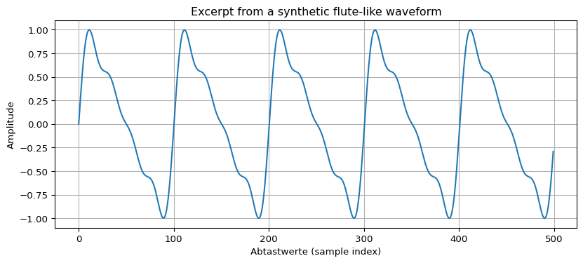
Consider a short excerpt from a recorded flute tone stored in a wavetable. Processing of such a sample typically involves:

• Looping a suitable part of the waveform to obtain sustained tones,
• Pitch shifting to play different notes from the same sample,
• Multi-sampling (using several samples for different pitch/velocity ranges),
• Enveloping (applying an amplitude envelope over time),
• Filtering (spectral shaping).

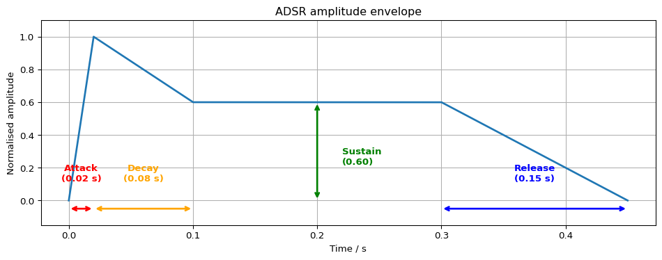
A commonly used amplitude envelope model is the Attack–Decay–Sustain–Release (ADSR) envelope. It describes the envelope with four key points, giving a simple approximation of the instrument’s transient behaviour. For more realism, one can additionally store explicit transient segments before and after the loop.

1.3 Looping in Wavetable Synthesis

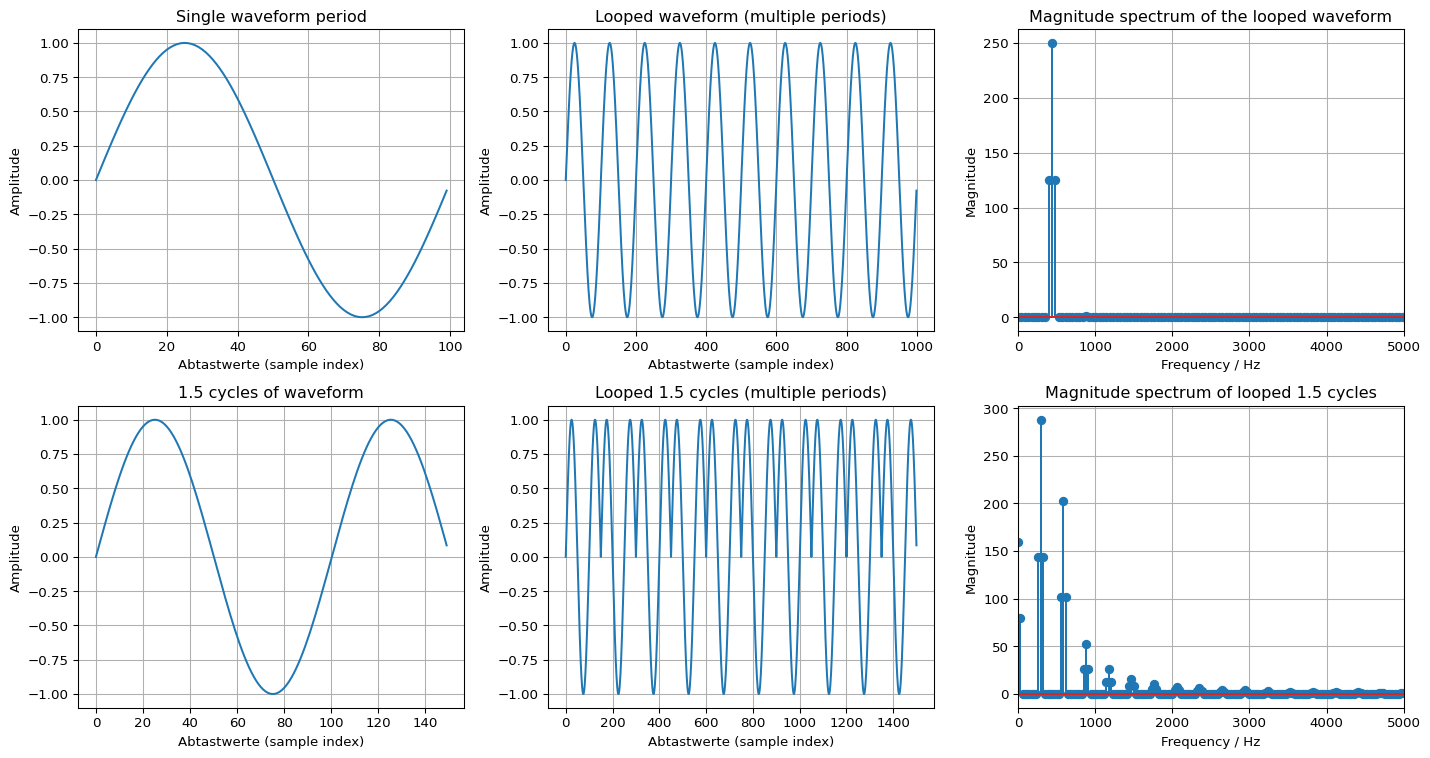
To create sustained tones from a finite-length recording, one typically selects a region of the waveform and loops it (repeats it) while a key is held.

• The loop length is often chosen as the duration of the fundamental period (or an integer multiple), so that the loop joins smoothly.
• For vibrato (frequency modulation of the pitch) or tremolo (modulation of the amplitude), the loop length can match the period of the slow variation.

Below is a simple example that demonstrates looping of a single-period waveform and shows the resulting spectrum.

1.4 Pitch Shifting

• To save memory space, only selected notes of an instrument are stored.
• Notes which have not been stored are reproduced from the stored ones by pitch shifting.

1.4.1 Trivial pitch shifting:

• Increase the pitch by subsampling (double, triple or quadruple the pitch)
• But: audible shifting of the formants by one, two, three octaves

1.4.2 Difficult: pitch shifting by a semitone

• 2^{1/12} = 1.0595 times the original pitch

1.4.3 Basic principles:

• Asynchronous and synchronous pitch shifting

1.5 Pitch Shifting: Asynchronous

Advantages	Disadvantages
Arbitrary shift by continuous variation of the clock frequency (asynchronous)	For polyphonic instruments: different sample rates for each channel
Simple circuitry (analog lowpass: switched capacitor filter)	For each channel one digital-analog converter
No digital post-processing	Adding different voices only by summation of analog signals

Applied in the first wavetable synthesizers until ca. 1985.

1.6 Pitch Shifting: Synchronous

1.6.1 Idea:

• Interpolation of the sample values in the wavetable
• Resampling with new sampling rate

1.7 Synchronous Pitch Shifting: Interpolation

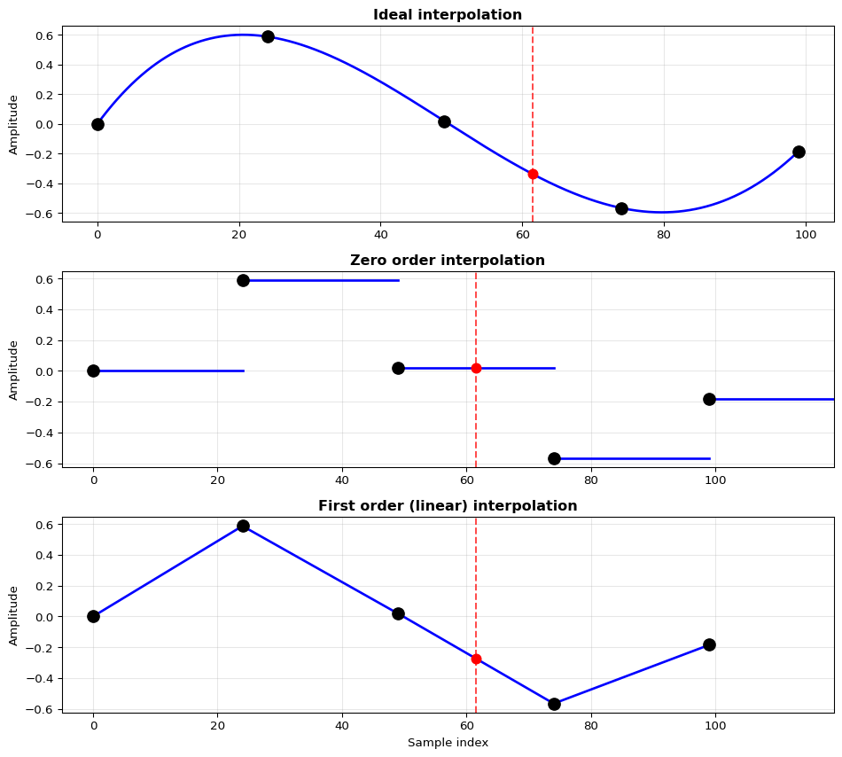
For zero-order or first-order interpolation, the interpolated value can be obtained from the neighbour values in a simple fashion.

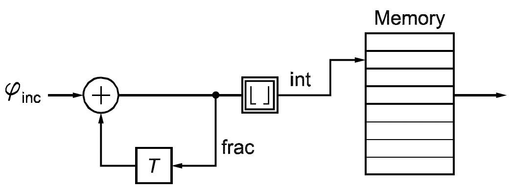
For fractional phase increment (e.g., 1.0595):

• Split the phase into two parts:
  • Integer part: addresses the wavetable (accumulated)
  • Fractional part: accumulated

The interpolated value is obtained from the neighbour values.

Synchronous Pitch Shifting

1.8 Zero Order Interpolation

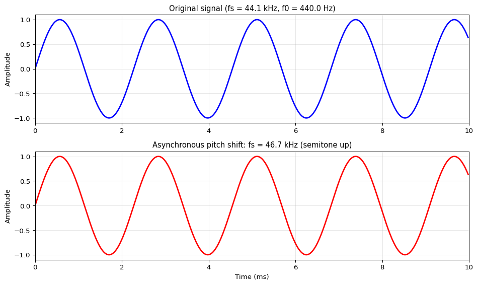
Increase the pitch by dropping samples Decrease the pitch by repeating samples

1.9 First Order Interpolation

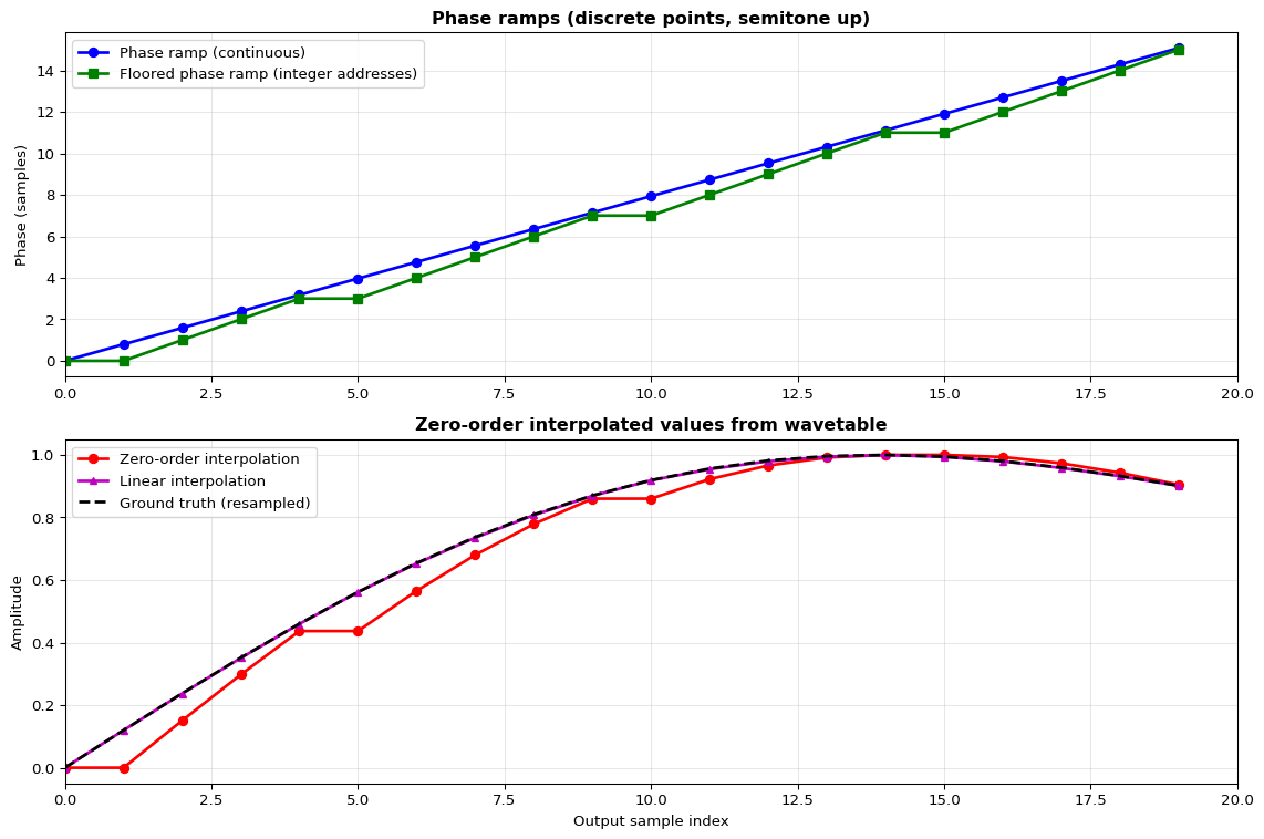
Calculation of the intermediate values by linear interpolation, e.g.,

y(1.0595) \approx y(1) \cdot (1 - 0.0595) + y(2) \cdot 0.0595

Linear interpolation gives good results for smooth functions.

1.10 Multisampling

1.10.1 Required Memory

To avoid errors, multidimensional multisampling is used.

Example: Multisample for a grand piano:

• 88 keys
• Separate wavetable for 8 velocity levels
• Each note: 2 minutes
• Each octave or quint

Total duration: almost a day!

Required memory: 1.8 GB

1.10.2 Realization

• Only the beginning of each wavetable resides in solid state memory
• The remainder is loaded from disc when required

1.10.3 Multidimensional Multisampling

• No more pitch shifting, no more looping
• Requires a large and fast disc and cache
• Dimensions: pitch, velocity, playing style

1.11 Wavetable Synthesis as Software Synthesizer

Required memory per instrument: several GB

1.11.1 Sound Examples: Gigastudio

• Harp
• Piano

1.11.2 Available Commercial Samples

• All kinds of individual instruments (Ableton’s Wavetable)
• Symphonic orchestra (Vienna Symphonic Library)
• Individual instruments and groups of instruments
• Vintage audio equipment
• Effect sounds
• And more

1.12 Summary: Wavetable Synthesis

So far: wavetable synthesis — reproduction of recorded sounds

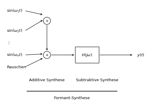
Two approaches:

1. High fidelity reproduction with high memory requirements (multidimensional multisampling)
2. Variability through looping and post-processing

1.12.1 Post-Processing Techniques

• Enveloping: ADSR envelope
• Filtering: spectral shaping
  • Time-invariant filters: lowpass, highpass, resonance filters (peak filters, shelving filters)
  • Time-variant filters: e.g., lowpass with variable bandwidth
    • Passband increases with velocity
    • Brighter sound with stronger key stroke

Sound synthesis by spectral shaping (subtractive synthesis)

2 Additive und subtractive synthesis

2.1 Additive synthesis

Compose a sound from single spectral components.

Theoretical foundation: Fourier series expansion

Synthesis:

y(t) = \Re\left\{ \sum_{\nu=-\infty}^{\infty} c_\nu \exp(j \nu \omega_0 t) \right\} = \sum_{\nu=0}^{\infty} a_\nu \cos(j \nu \omega_0 t + \varphi_\nu)

Realisation by a bank of parallel resonators.

Analysis (according to Fourier theory):

c_\nu = \frac{1}{T} \int_{t_0}^{t_0 + T} y(t)\,\exp(-j \nu \omega_0 t)\, dt, \qquad \omega_0 = \frac{2\pi}{T}

2.2 Subtractive synthesis

Filtering:

y(t) = h(t) * x(t), \qquad h(t) = \mathcal{F}^{-1}\{ H(j\omega) \}

Realisation by serial filters.