What an Observation Is Worth

Dependence, the posterior, and the cost that picks the estimate

Seeing one thing, learning another

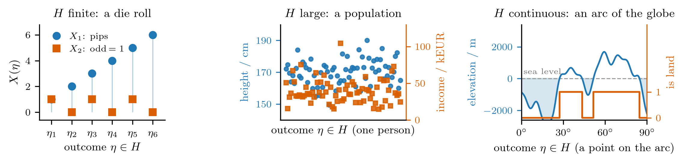
Three pairs, one question

Two readings of each of three experiments: pips and parity of a die, height and income of a person, elevation of a point and whether it is land.

In each case you are told one reading and asked about the other. What is the observation worth?

Guess before the pictures: parity for pips, height for income, elevation for land.

The plan for the week

Dependence. What one variable says about another lives in their joint law, and conditioning is how you read it off.

Inference with a prior. Model the unknown as random, and the observation turns the prior into a posterior. A cost then says which single number, or which decision, to report.

In the notes Joint Distributions and Marginals · Conditional Distributions · Functions of Two Random Variables · The Posterior · Cost, Risk, and Pointwise Minimization · Bayes Decision and Classification · Bayesian Estimation: MMSE and MAP · Two Scalar Problems: Fusion and Denoising

Dependence lives in the joint law

Events for a pair are regions of the plane
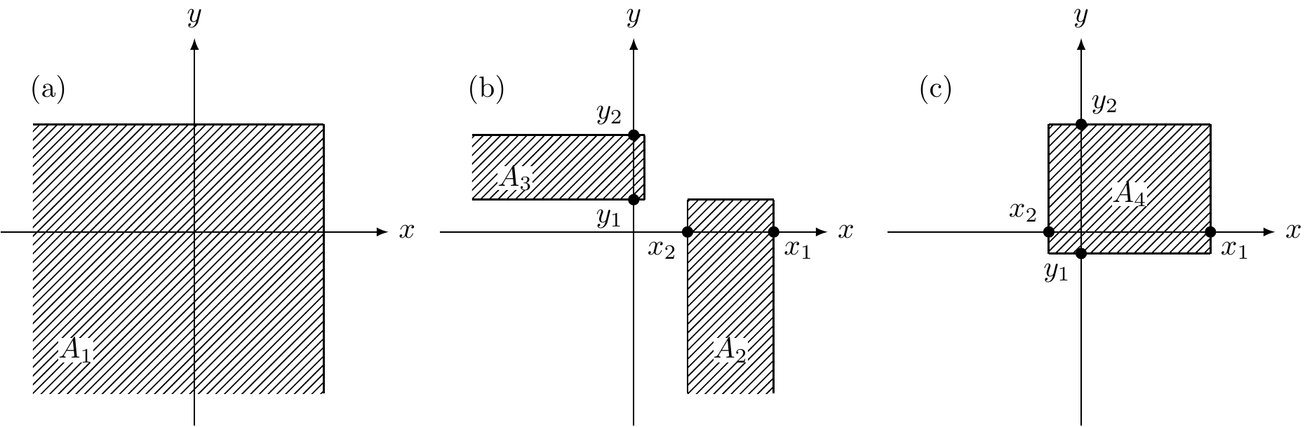
(a) The quadrant whose mass is the joint CDF. (b) Strips that constrain one variable only. (c) A rectangle, by inclusion–exclusion of four quadrants.

Joint CDF and density \[F_{XY}(x,y)=\Prob{X\le x,\ Y\le y},\qquad f_{XY}(x,y)=\frac{\partial^2F_{XY}(x,y)}{\partial x\,\partial y}.\]

The three pairs, as joint laws
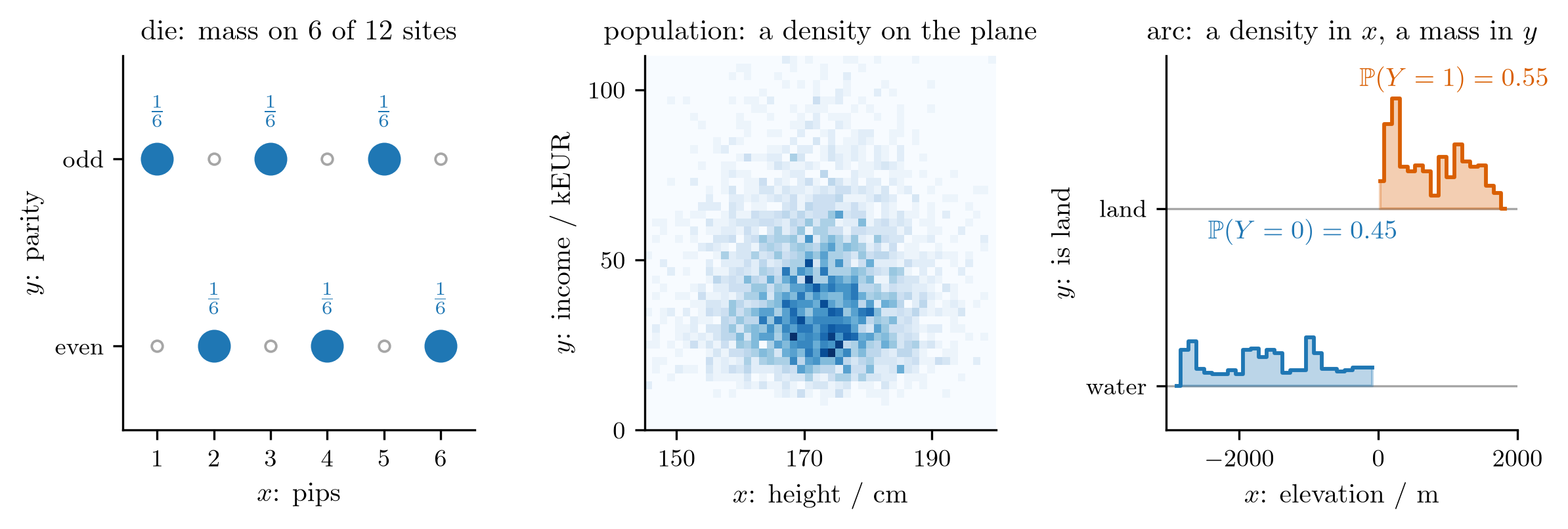
Mass on a lattice, a density on the plane, and a density in \(x\) carrying a mass in \(y\).

The die and the terrain put mass only where the two readings agree; the population has no such structure. Discrete, continuous, or one of each: the object is the same, a nonnegative assignment of total mass one to the plane.

Marginals throw the dependence away

\[f_X(x)=\int f_{XY}(x,y)\dd y,\qquad f_Y(y)=\int f_{XY}(x,y)\dd x .\]
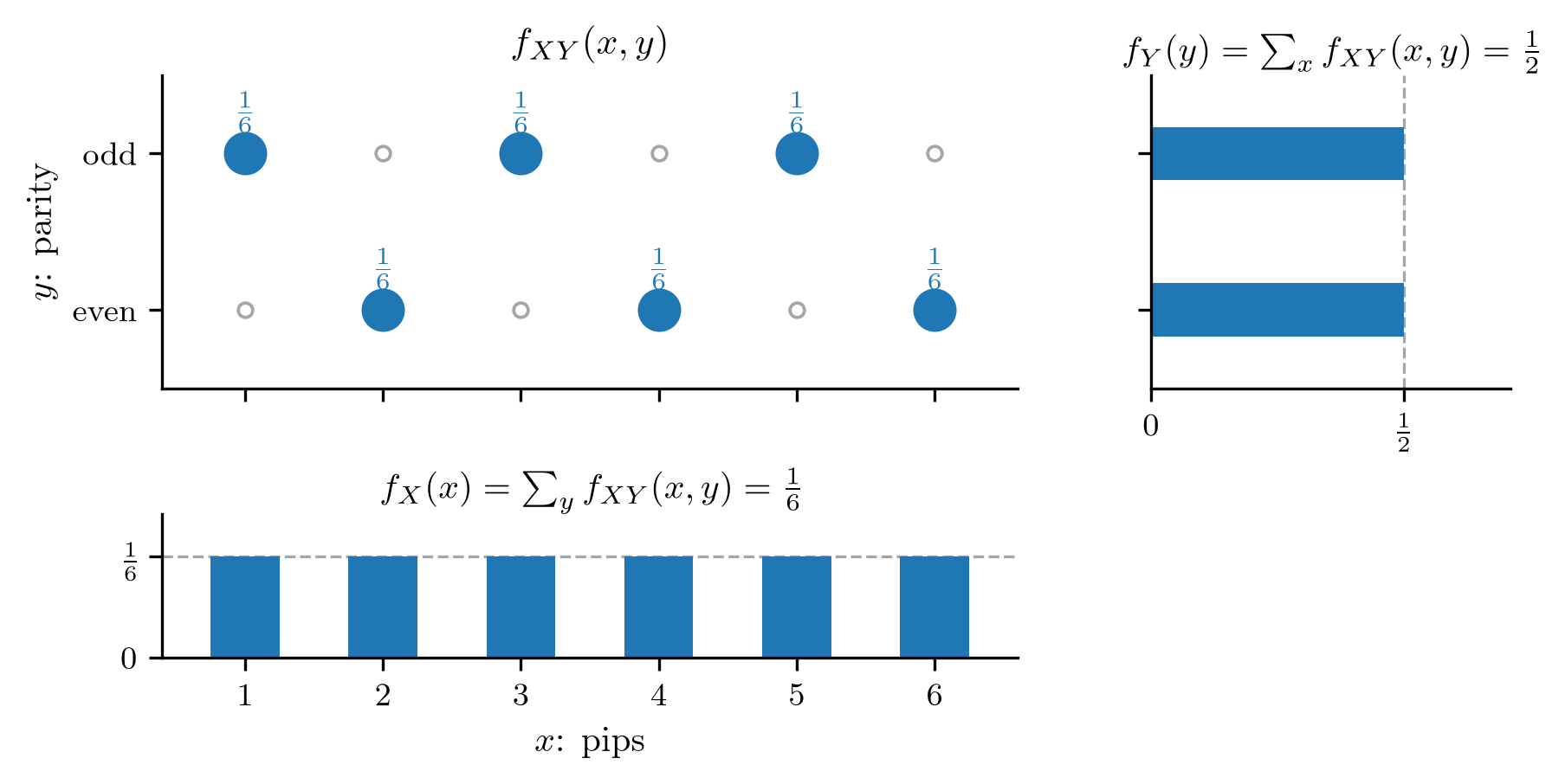
Summing the die’s joint law over one coordinate returns the law of the other.

A fair die and a fair coin, and no trace of the fact that the mass sat only where pips and parity agree. All of the dependence was in the joint.

Same marginals, three different worlds
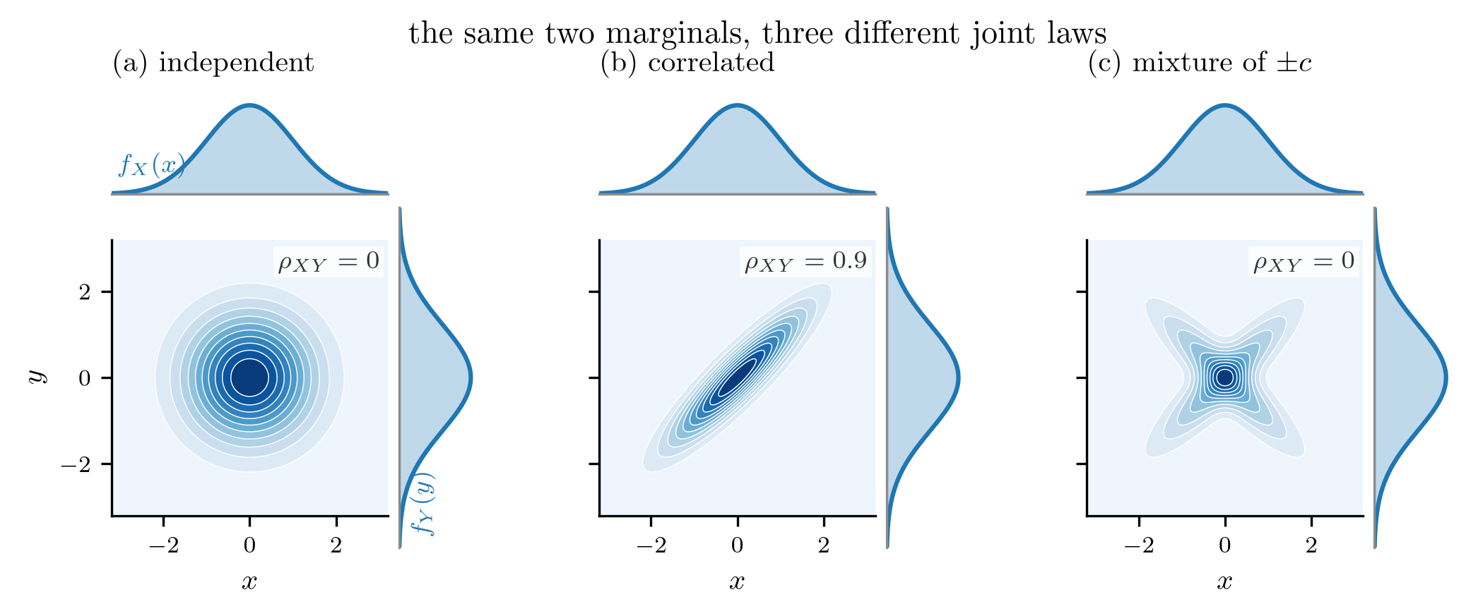
Three pairs with identical standard Gaussian marginals: independent, tilted along one diagonal, and a mixture tilted along both.

Observing \(X\) says nothing about \(Y\) in the first, pins \(Y\) to a band in the second, and in the third says “near \(+x\) or near \(-x\)” without choosing. Only the joint density tells them apart.

Independence, and what it buys

Independence \[f_{XY}(x,y)=f_X(x)\,f_Y(y).\]

Sums split always: \(\E{aX+bY}=a\E{X}+b\E{Y}\) needs only a joint law to exist.

Products split only under independence: \(\E{g(X)h(Y)}=\E{g(X)}\E{h(Y)}\).

The asymmetry is worth remembering. A sum of dependent terms is still easy to average; a product of them is not.

Conditioning: the slice through the joint

Conditional density \[f_{Y\mid X}(y\mid x)=\frac{f_{XY}(x,y)}{f_X(x)}:\] take the slice of the joint at the observed \(x\) and renormalize it.

Independence is exactly \(f_{Y\mid X}(y\mid x)=f_Y(y)\): the slice looks like the whole.

An observation is worth something exactly when the conditional differs from the marginal. The three pairs show the three possibilities.

Worth one bit

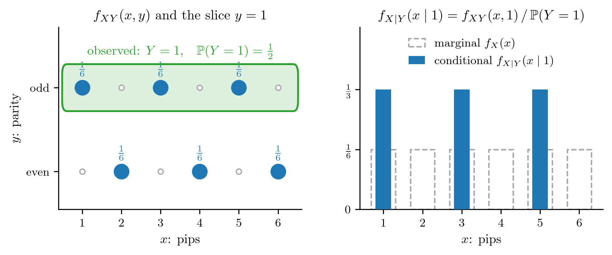
Keep the slice “odd”, divide by its mass \(\tfrac12\), read off the conditional law of the pips.

Odd rules out three faces and doubles the weight of the other three. A guess of the face gets better, but not certain.

Worth nothing
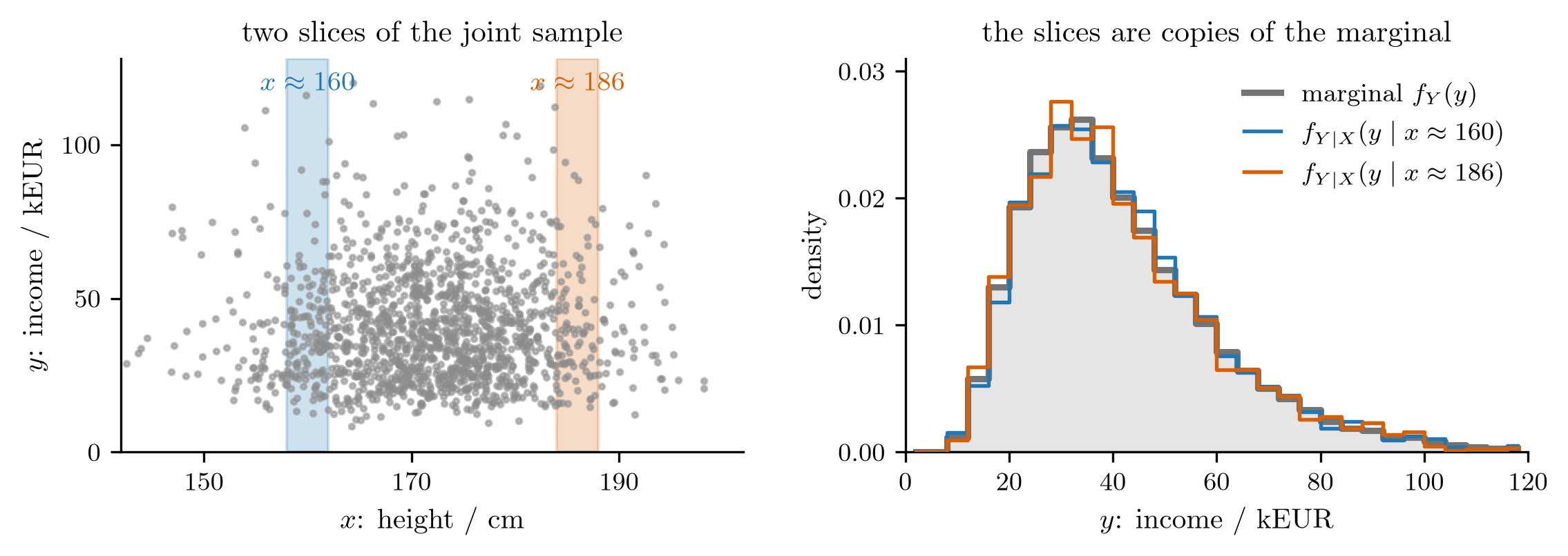
The income density inside two slices of height, against the income of the whole population.

Short slice, tall slice, everyone: one curve. The height is measured, and the estimate of the income does not move. That is independence, seen from the conditioning side.

Worth everything
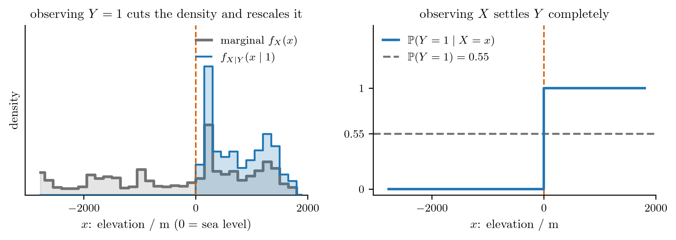
Left: elevation given that the point is land. Right: land given the elevation.

The elevation settles the land question outright: the probability is \(0\) below sea level and \(1\) above. The other way round, one bit only cuts the elevation density at sea level. Dependence is symmetric; what each direction is worth is not.

Bayes’ rule for densities

The joint can be sliced either way, \(f_{XY}=f_{Y\mid X}\,f_X=f_{X\mid Y}\,f_Y\), so

Bayes’ rule \[f_{Y\mid X}(y\mid x)=\frac{f_{X\mid Y}(x\mid y)\,f_Y(y)}{f_X(x)},\qquad f_X(x)=\int f_{X\mid Y}(x\mid y)\,f_Y(y)\dd y .\]

Turning the conditional around is the whole of Bayesian inference. The second part of the week is this formula, used with intent.

Two variables in, one out

A map deforms the plane

A function of two variables moves probability mass around the plane; the density picks up the Jacobian of the map, the ratio by which it stretches area.
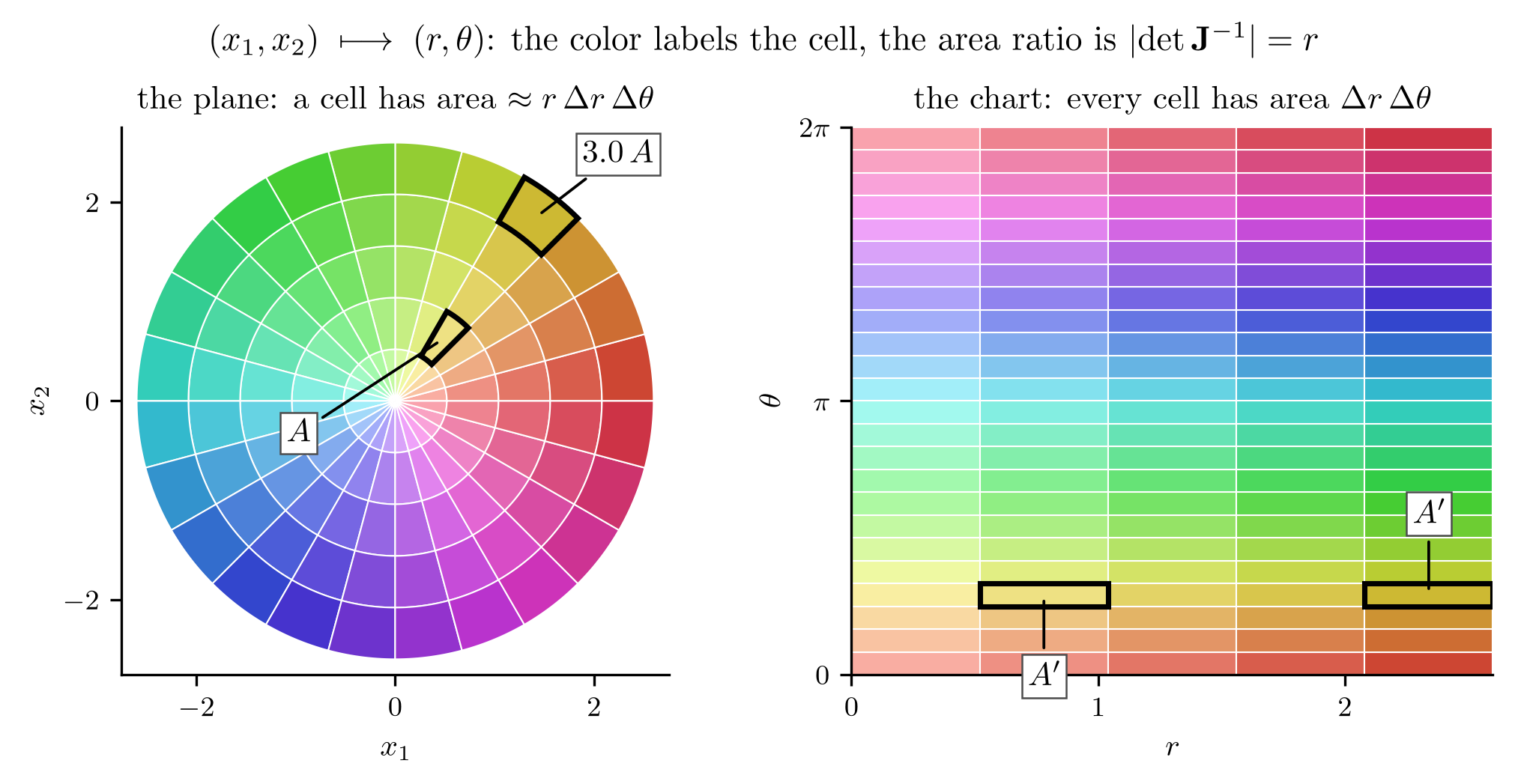
The polar map as a deformation: color labels each cell, and equal cells in the chart have areas proportional to their radius in the plane.

The notes have the change-of-variables formula. Three results from it matter for signals, and the next three slides show them.

A sum is a shear
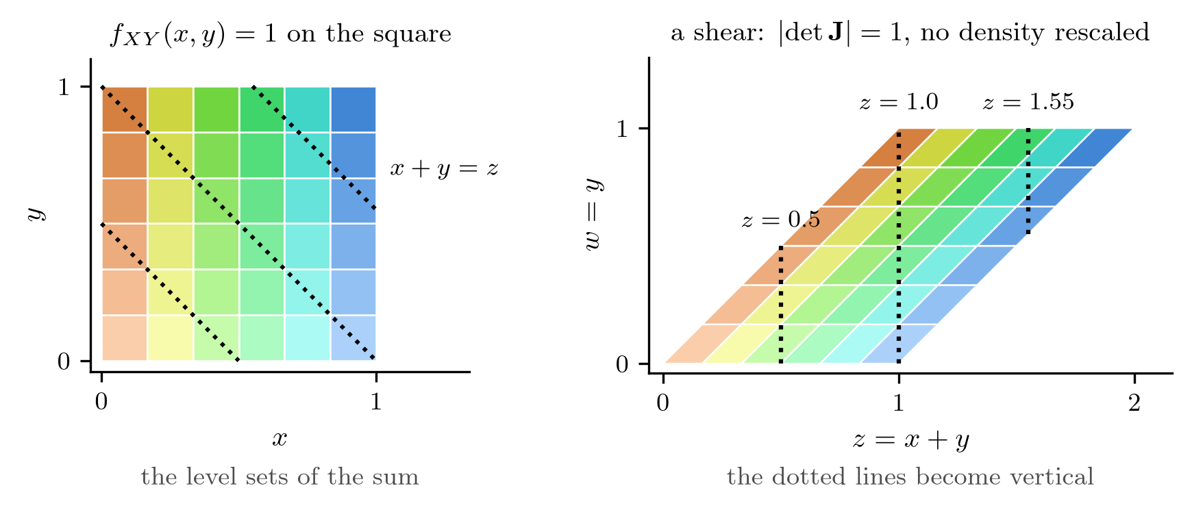
The sum of two independent uniforms as the shear \((x,y)\mapsto(x+y,\,y)\): lines of constant sum become vertical, ready to be integrated out.

Shear, then marginalize: that is where the convolution of densities for an independent sum comes from, the smoothing step of the first week drawn as a map.

The envelope of a Gaussian pair is Rayleigh
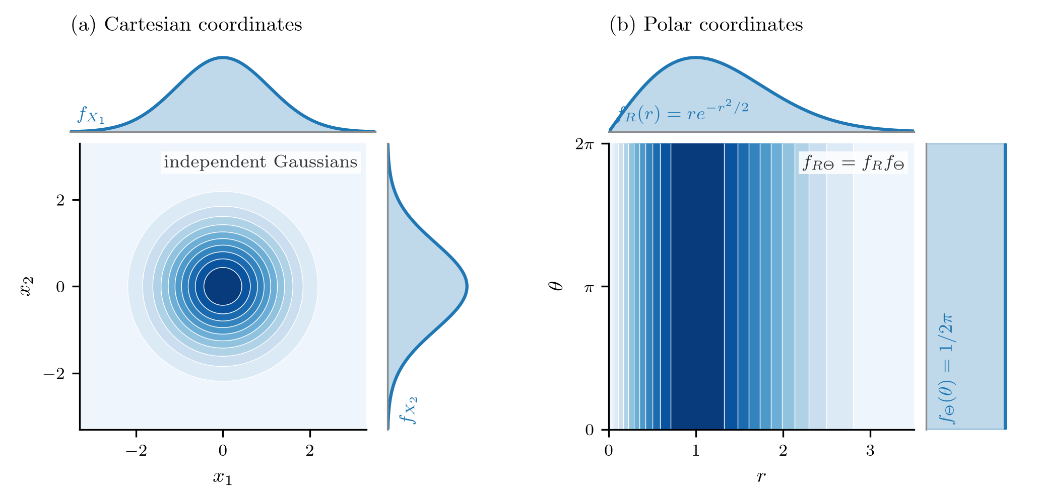
An isotropic Gaussian pair mapped to radius and angle: the radius is Rayleigh, the angle uniform, and the two are independent.

The magnitude of complex Gaussian noise, which is what an envelope detector sees, is Rayleigh distributed. Read backwards (Box–Muller), two uniforms make two Gaussians.

Two uniforms make two Gaussians
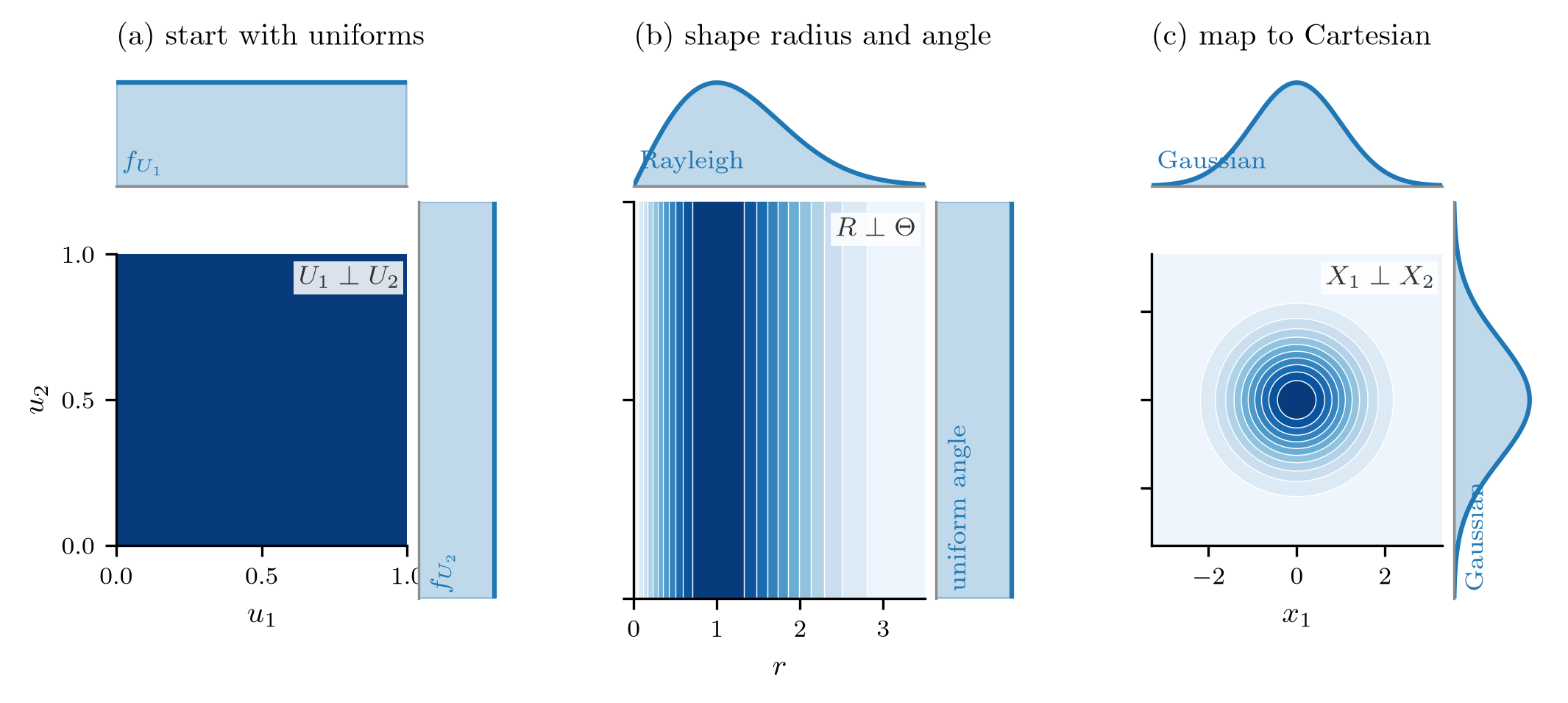
Box–Muller: two independent uniforms become a Rayleigh radius and a uniform angle, then an isotropic Gaussian pair.

The envelope construction read backwards. This is how Gaussian noise is generated in software from a uniform random-number generator.

Sums and ratios
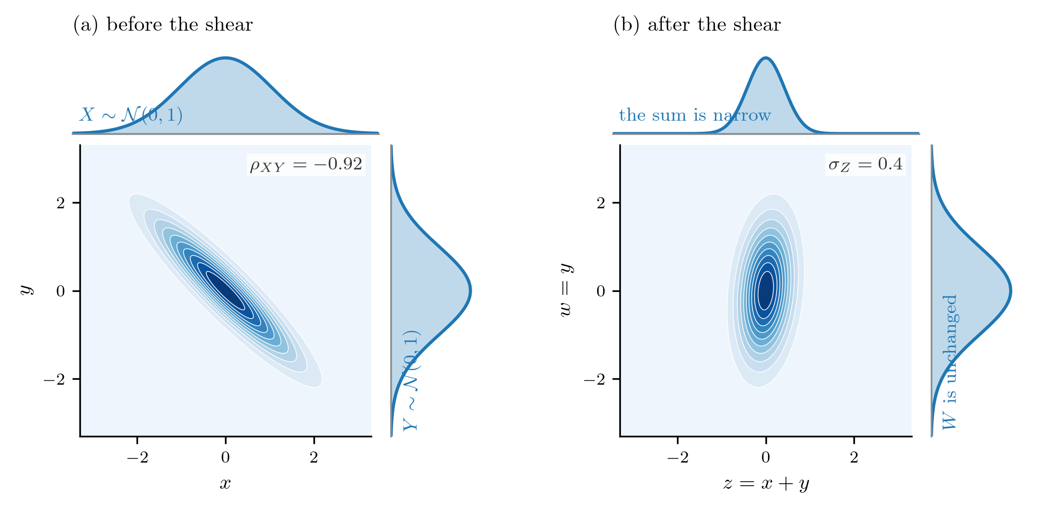
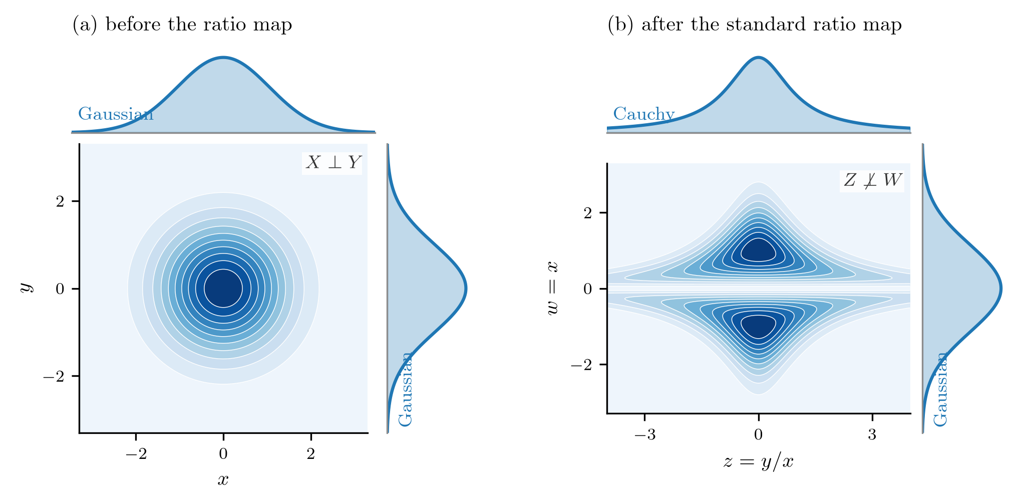
A dependent sum: negatively dependent Gaussians nearly cancel, so the sum is narrow. A ratio of two Gaussians: the retained coordinate stays Gaussian, the ratio is Cauchy.

Dependence can make a sum smaller than either term: variances add only for independent terms. And the Cauchy law of the first week is just the ratio of two ordinary Gaussians.

The posterior

Model the unknown as random

Give the unknown \(Y\) a prior \(f_Y(y)\), and let the observation depend on it through \(f_{X\mid Y}(x\mid y)\). Now a joint law exists, and conditioning is inference:

Posterior \[f_{Y\mid X}(y\mid x)=\frac{f_{X\mid Y}(x\mid y)\,f_Y(y)}{f_X(x)} \qquad\propto\qquad \text{likelihood}\times\text{prior}.\]

Last week’s semicolon, \(f(x;\phi)\), has become a bar, \(f_{X\mid Y}(x\mid y)\). The formula for the likelihood is the same; what changed is that \(Y\) now has a law of its own.

Model the unknown as random

Bayesian estimation as a signal flow: the unknown is now uppercase, random, with a known prior; the family has become a conditional density.

Against last week’s picture, one thing changed: the node on the left acquired a law.

Prior times likelihood

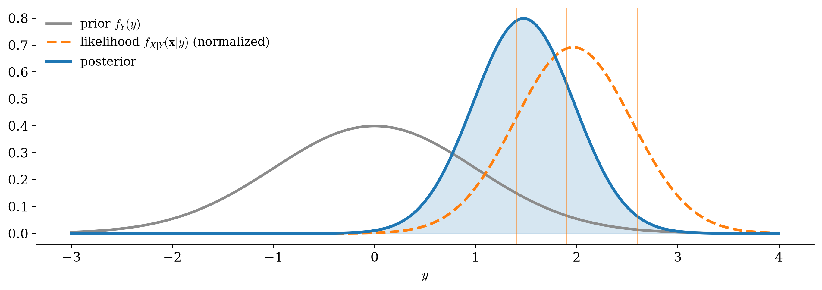
Figure 1: A Gaussian prior on Y, the likelihood of three noisy observations, and their normalized product, the posterior.

The posterior sits between prior and data, narrower than either: each source of information sharpens the other. The data’s pull grows with every observation; the prior’s does not.

A proportion, from a flat prior

How much of the Earth is land? Drop random points on a globe and record land or water. With a flat prior on the land fraction \(\phi\) and \(s\) land points out of \(N\), \[f_{\Phi\mid\mathbf X}(\phi\mid\mathbf x)\propto\phi^{s}(1-\phi)^{N-s},\qquad 0\le\phi\le1 .\]
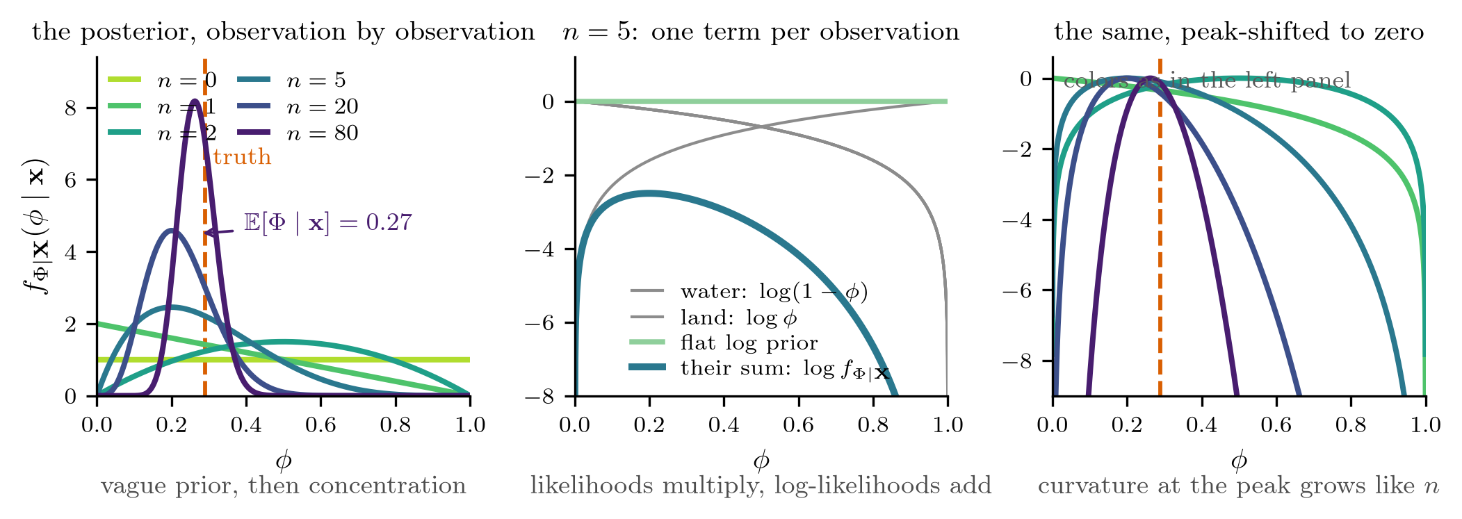
Left: the posterior after 0, 1, 2, 5, 20 and 80 points. Middle: the log-posterior as a sum of one term per observation. Right: the log-posteriors, sharpening in proportion to \(N\).

Watching a prior become a posterior

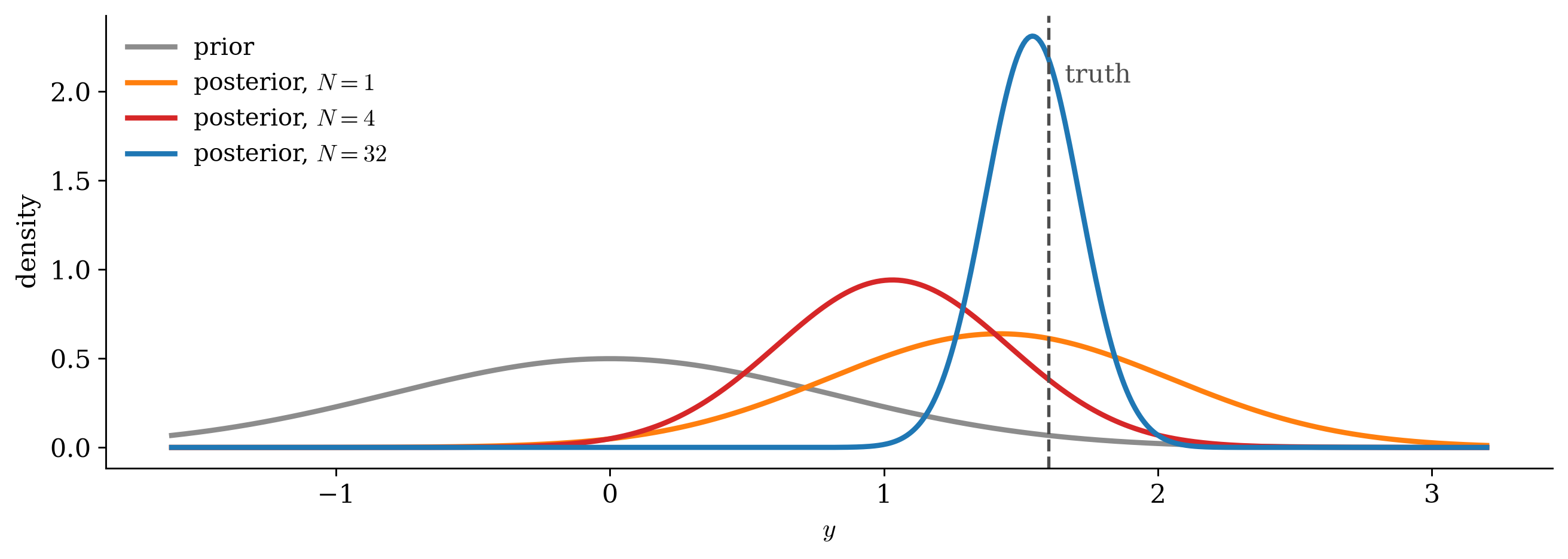
Figure 2: A Gaussian prior updated by 1, 4 and 32 noisy observations of the same unknown.

With one observation the prior still dominates; by \(N=32\) it hardly matters. The prior never has to be switched off: the data retire it on their own.

The conditional mean is an estimator

Conditional mean \[\E{Y\mid x}=\int y\,f_{Y\mid X}(y\mid x)\dd y\]

At the observed \(x\) this is an ordinary mean of an ordinary density. Read as a function of the random \(X\), \(\E{Y\mid X}\) is itself a random variable, with the tower property \(\E{\E{Y\mid X}}=\E{Y}\).

With no data the best constant guess was the prior mean \(\E{Y}\). Observation replaces it by the conditional mean: start at the prior mean and let the data supply a correction.

The cost picks the answer

The posterior is the answer; the estimate is a summary

A usable answer is one number, or one decision. Which one follows from what a mistake costs, \(\calC(y,\widehat y)\ge0\).

Conditional risk and Bayes risk \[R(\widehat y\mid x)=\int\calC(y,\widehat y)\,f_{Y\mid X}(y\mid x)\dd y,\qquad R(\widehat y(\cdot))=\iint\calC(y,\widehat y(x))\,f_{XY}(x,y)\dd y\dd x .\]

The first belongs to this data set and a candidate answer; the second to the rule, before any data are seen. It is the number by which two procedures are compared.

Minimize one slice at a time

Pointwise minimization The rule with the smallest Bayes risk minimizes the conditional risk separately at each observed \(x\).
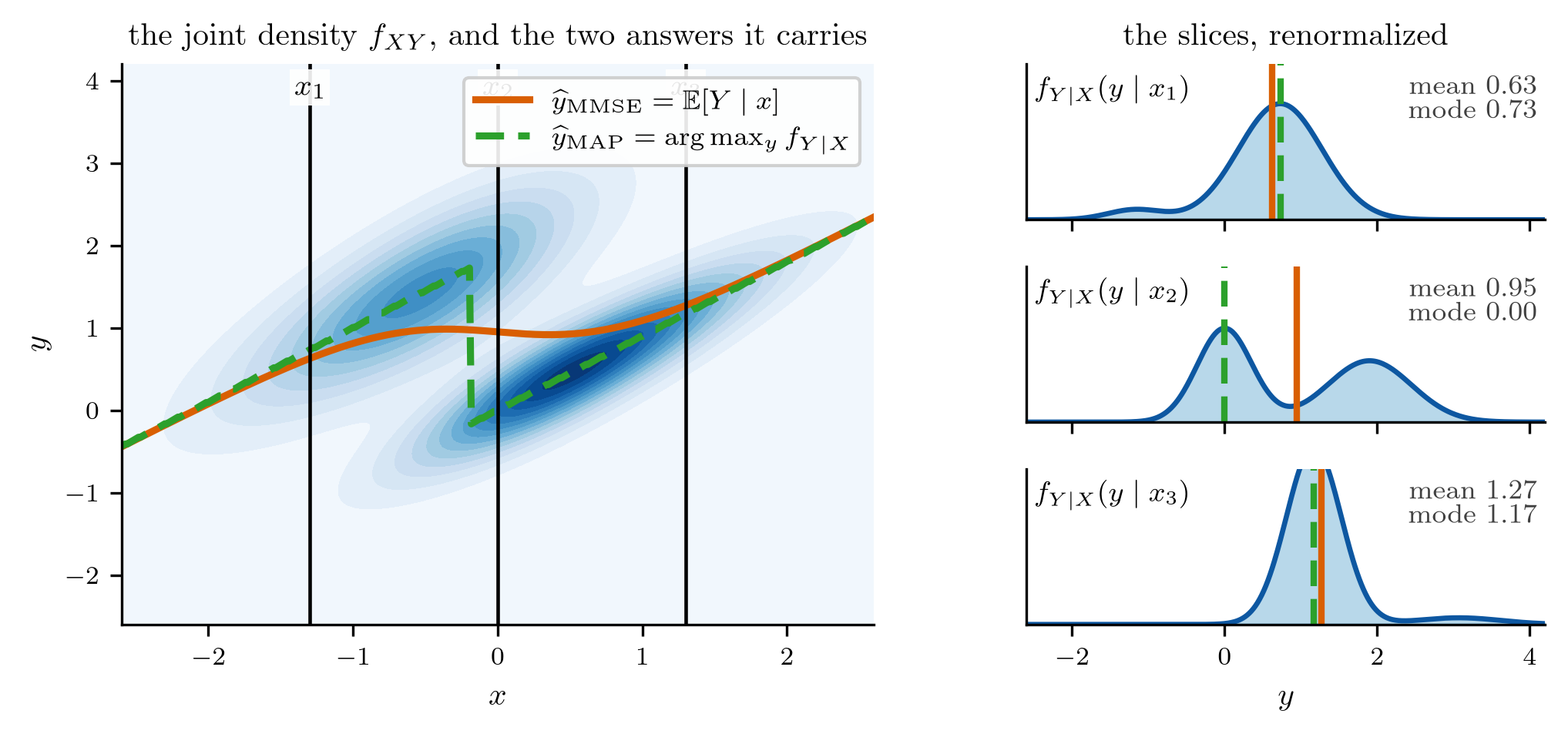
Left: a joint density with the posterior mean and mode as functions of \(x\). Right: three slices, each its own scalar problem. At \(x_2\) the posterior is bimodal and the mean falls in the trough.

An optimization over all possible rules collapses into one scalar problem per observation. And a mean need not be a plausible value.

Deciding with priors and costs

Two hypotheses with prior probabilities \(P_0,P_1\), and cost \(C_{ij}\) for deciding \(i\) when \(j\) is true. Minimizing pointwise:

Bayes decision rule Decide \(H_1\) where \[\Lambda(\mathbf x)=\frac{f_{X\mid H}(\mathbf x\mid H_1)}{f_{X\mid H}(\mathbf x\mid H_0)} \;>\;\frac{P_0\,(C_{10}-C_{00})}{P_1\,(C_{01}-C_{11})}.\]

The same statistic as Neyman–Pearson. A false-alarm budget and an average cost choose the same test and differ only in the threshold.

Deciding with priors and costs

Bayes decision as a signal flow: detection with a prior probability on each hypothesis.

Priors and costs pick the operating point
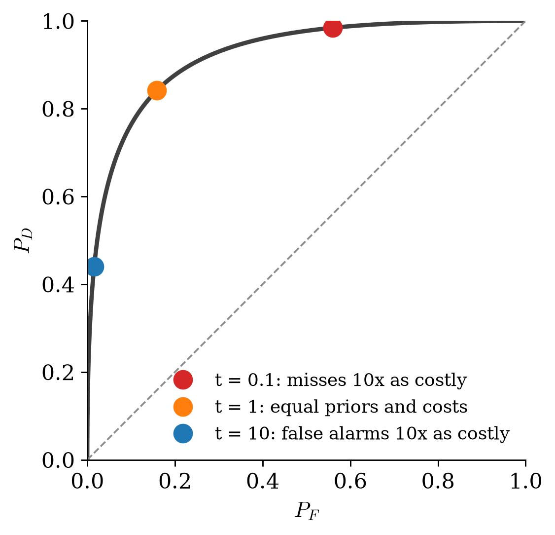
Figure 3: A known level ±1 in unit Gaussian noise. The ROC is fixed by the data; the Bayes threshold t = P0 C_FA / (P1 C_miss) picks the point on it.

The data decide the curve; what you believe and what you stand to lose decide where on it you sit. A smoke alarm and a spam filter sit at opposite ends.

Reading it as odds

The likelihood ratio updates the prior odds \[\frac{\Prob{H_1\mid\mathbf x}}{\Prob{H_0\mid\mathbf x}}=\Lambda(\mathbf x)\,\frac{P_1}{P_0}.\]

  • equal costs: pick the larger posterior, a MAP decision;
  • equal priors too: pick the larger likelihood, an ML decision.

\(\Lambda\) is exactly the factor by which the data move your belief. Everything else in the threshold is what you believed and what you stand to lose.

More than two classes

With a discrete label \(Y\in\set{1,\dots,M}\) the same pointwise rule answers, at each \(\mathbf x\), with the label of smallest expected cost; with equal costs, the largest posterior:

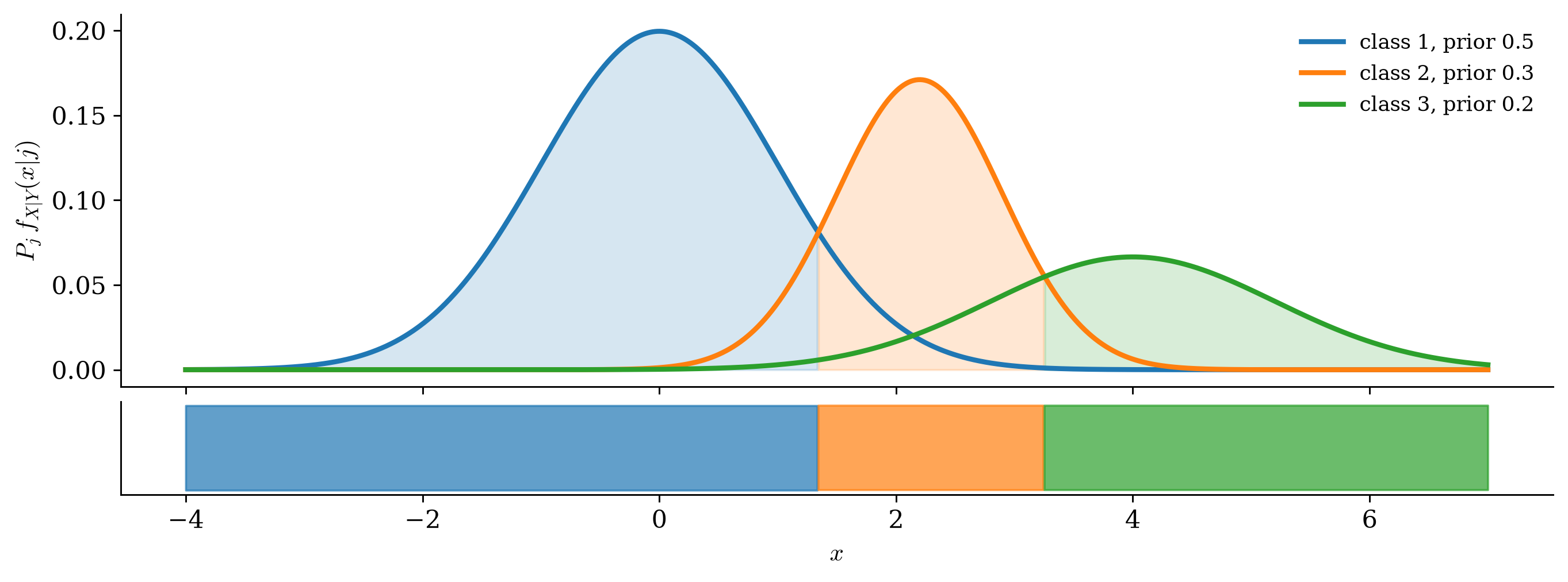
Bayes classifier \[\widehat y(\mathbf x)=\argmax_j\ P_j\,f_{X\mid Y}(\mathbf x\mid j).\]

The best any classifier can do when the laws are known. Every learned classifier is an attempt to approximate it from data.

Three classes, drawn

Figure 4: Three classes with priors 0.5, 0.3, 0.2 and Gaussian likelihoods. Top: the weighted densities P_j f(x|j). Bottom: the class the Bayes classifier picks at each x.

At each \(x\) the largest weighted density wins. The boundaries sit where two curves cross, shifted toward the class that is less likely a priori.

Estimating: squared error gives the mean

For \(\calC=(y-\widehat y)^2\) the conditional risk is a quadratic in \(\widehat y\): \[\frac{\dd}{\dd\widehat y}\int(y-\widehat y)^2f_{Y\mid X}(y\mid x)\dd y =-2\paren{\E{Y\mid x}-\widehat y}=0 \quad\Longrightarrow\quad\widehat y_{\text{MMSE}}=\E{Y\mid x}.\]

The best estimate there is Over all data, \(\E{Y\mid X}\) minimizes \(\E{(Y-g(X))^2}\) over every function \(g\), linear or not. Much of this course computes it, or an approximation to it.

How good is the best estimate?

The error of \(\E{Y\mid X}\) is what the posterior still does not know, averaged over the data:

Law of total variance \[\E{(Y-\E{Y\mid X})^2}=\E{\Var{Y\mid X}},\qquad \Var{Y}=\underbrace{\E{\Var{Y\mid X}}}_{\text{left unexplained}}+\underbrace{\Var{\E{Y\mid X}}}_{\text{explained by }X} .\]

The prior spread splits into the part the observation explains and the part it cannot. For the three pairs: the population explains nothing, the terrain everything, the die something in between.

The error is uncorrelated with everything you saw

Orthogonality of the MMSE error \[\E{\paren{Y-\E{Y\mid X}}\,g(X)}=0\qquad\text{for all } g .\]

Otherwise adding a multiple of \(g(X)\) would lower the error. By the tower property the expectation is \(\E{\paren{\E{Y\mid X}-\E{Y\mid X}}g(X)}=0\).

Optimal means: nothing left in the data that could still explain the error. This is the characterization, not a side property.

Hit or miss gives the mode

For a cost that is \(0\) inside a tiny window around the truth and \(1\) outside, the best answer is the value the posterior makes most probable:

MAP estimate \[\widehat y_{\text{MAP}}=\argmax_y\ f_{X\mid Y}(x\mid y)\,f_Y(y).\]

MAP is maximum likelihood plus a prior. Caveat: a mode moves under a change of variables; the mean does not.

Mean or mode: it matters which

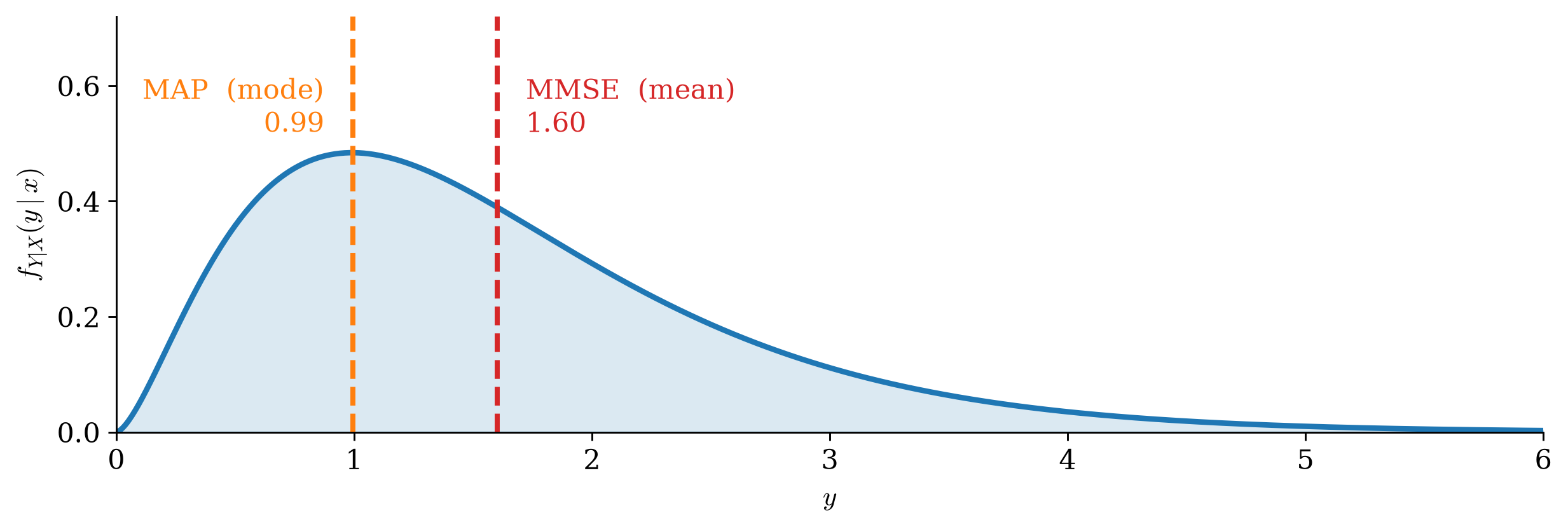
Figure 5: A skewed posterior, with its mode (MAP) and its mean (MMSE).

For a symmetric, single-peaked posterior they coincide. Away from symmetry they answer different questions: the most probable value against the value with least squared error.

One framework, three questions

\[\widehat y_{\text{Bayes}}(x)=\argmin_{\widehat y}\int\calC(y,\widehat y)\,f_{Y\mid X}(y\mid x)\dd y\]

unknown cost answer
two hypotheses hit or miss, with costs likelihood-ratio test
\(M\) classes costs \(C_{ij}\) Bayes classifier
a continuum squared error posterior mean
a continuum hit or miss posterior mode

Detection and estimation are one problem, differing only in the cost and in whether the unknown is discrete or continuous.

Two scalar problems

One unknown, several noisy looks

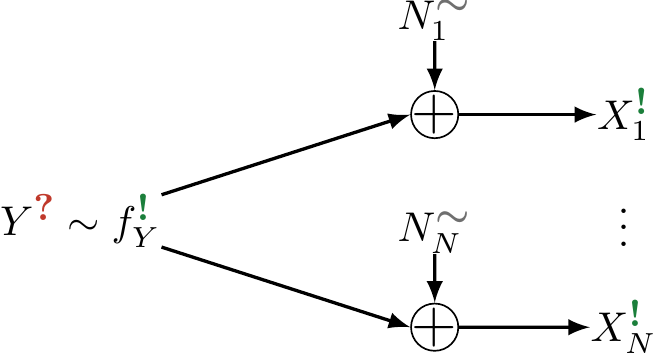
\(X_k=Y+N_k\), the noises independent of each other and of \(Y\). The log-posterior is a sum: \[\log f_{Y\mid\mathbf X}(y\mid\mathbf x)=\underbrace{\log f_Y(y)}_{\text{prior}} +\underbrace{\sum_{k}\log f_{N_k}(x_k-y)}_{\text{one term per measurement}}+\text{const}.\]

Everything below is this line under different choices of prior and noise. Fusion adds likelihood terms; denoising adds an informative prior as one more term.

One unknown, several noisy looks

Fusion as a signal flow: one sought unknown with a prior, seen through \(N\) channels, each adding its own noise.

Fusing two unequal sensors

Two thermometers with independent Gaussian errors \(\sigma_1^2,\sigma_2^2\) and no prior preference. Completing the square:

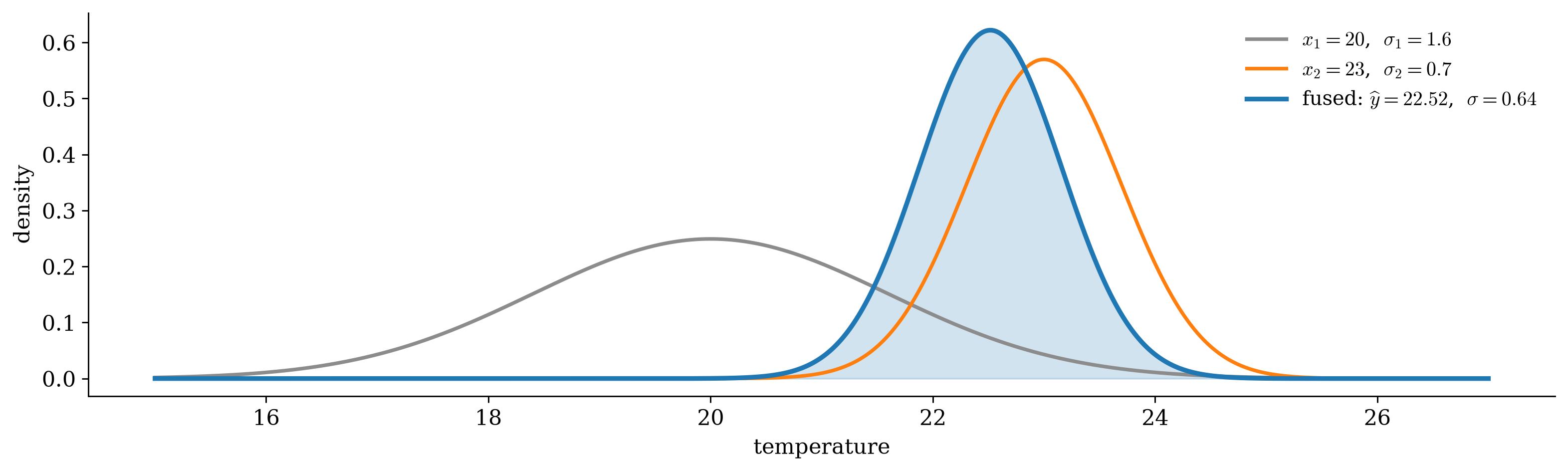
Precision-weighted fusion \[\frac{1}{\sigma_{\text{post}}^2}=\frac{1}{\sigma_1^2}+\frac{1}{\sigma_2^2},\qquad \widehat y=\sigma_{\text{post}}^2\paren{\frac{x_1}{\sigma_1^2}+\frac{x_2}{\sigma_2^2}} .\]

Fusing two unequal sensors

Figure 6: Two independent readings and the fused posterior.

Precisions add, and the estimate is the precision-weighted average: pulled toward the sharper reading, never worse than either. A useless sensor drops out by itself.

Denoising from \(N\) samples: shrink toward the prior

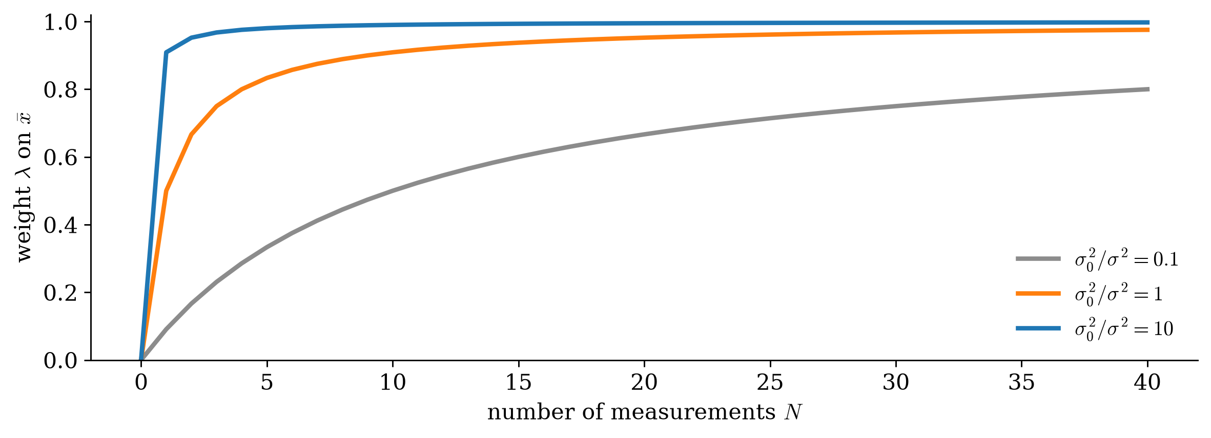
Shrinkage toward the prior Prior \(\Gauss(m_0,\sigma_0^2)\), \(N\) measurements with noise \(\sigma^2\): \[\widehat y=\lambda\,\overline x+(1-\lambda)\,m_0,\qquad \lambda=\frac{N\sigma_0^2}{\sigma^2+N\sigma_0^2}.\]

Few or noisy data: \(\lambda\approx0\), trust the prior. Many or clean data: \(\lambda\to1\), trust the sample mean. The prior acts as \(\sigma^2/\sigma_0^2\) extra measurements, all reading \(m_0\).

The posterior is Gaussian, so its mean and mode agree: this one formula is the MMSE and the MAP estimate at once.

How fast the data take over

Figure 7: The weight λ on the sample mean against the number of measurements, for three prior-to-noise ratios.

A vague prior (\(\sigma_0^2\gg\sigma^2\)) is overruled by the first measurement; a confident one needs many. Either way the weight goes to one: with enough data every reasonable prior agrees.

One observation: the shrinkage factor
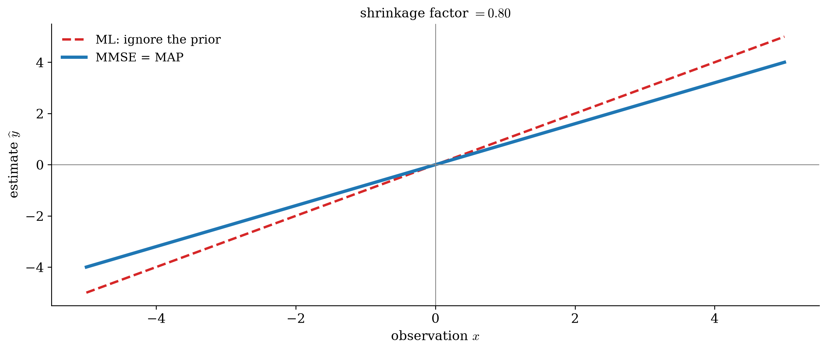
The shrinkage factor Observe \(X=Y+N\) once, prior \(\Gauss(0,\sigma_Y^2)\): \[\widehat y_{\text{MMSE}}=\widehat y_{\text{MAP}}=\frac{\sigma_Y^2}{\sigma_Y^2+\sigma_N^2}\,x .\]

One observation: the shrinkage factor

Figure 8: Estimate against observation, for \(\sigma_Y = 2\) and \(\sigma_N = 1\).

The estimate shrinks the observation by exactly the fraction of the observed power that is signal.

A sparse prior pulls mean and mode apart
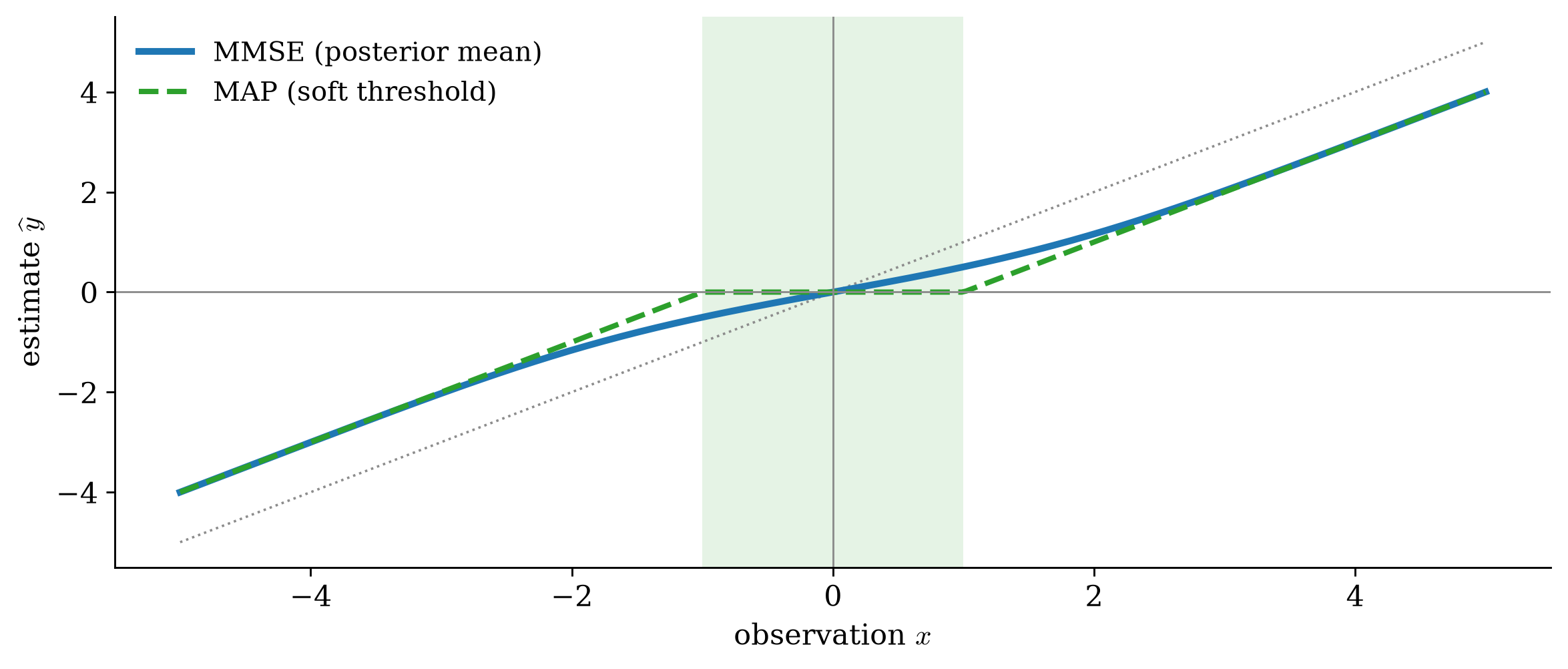
A signal that is mostly zero has a Laplacian prior, \(f_Y(y)\propto e^{-\abs{y}/b}\). MAP minimizes \((x-y)^2/2\sigma^2+\abs{y}/b\):

Soft thresholding \[\widehat y_{\text{MAP}}=\sign(x)\,\max\paren{\abs{x}-\sigma^2/b,\ 0}.\]

A sparse prior pulls mean and mode apart

Figure 9: Posterior mean and mode under a Laplacian prior, Gaussian noise \(\sigma = 1\), \(b = 1\).

MAP sets every small observation exactly to zero; the mean only shrinks smoothly. A Gaussian prior is a quadratic penalty and gives a linear estimator; the Laplacian’s \(\abs{y}\) penalty is the origin of every sparse-recovery method.

The trade of assumptions

estimator assumes needs
MMSE, MAP the full joint law the posterior
ML the likelihood only \(f_{X\mid Y}\)
restricted to a form (e.g. linear) less fewer quantities
fitted to data nothing about the law a training set

Read top to bottom: more assumptions buy better performance when they hold; fewer are hungrier for data but survive being wrong. The Gaussian is the one model where the cheap restricted forms lose nothing.

Outlook: denoising without knowing the prior

Tweedie’s formula For Gaussian noise \(X=Y+N\), \(N\sim\Gauss(0,\sigma^2)\), and any prior: \[\E{Y\mid X=x}=x+\sigma^2\,\frac{\dd}{\dd x}\log f_X(x).\]

It needs only the density of the observations, which can be learned from data, and not the prior.

It is the identity modern diffusion and score-based image denoisers are built on: the posterior mean of this week, computed by a network that has learned \(\log f_X\).

Recap

This week

  1. What an observation is worth lives in the joint law. Conditioning reads it off; it is worth something exactly when the conditional differs from the marginal.
  1. With a prior, inference is conditioning: the posterior is the complete answer, and the cost picks the summary. Squared error gives the posterior mean \(\E{Y\mid X}\), the best estimate there is; hit-or-miss gives the mode, and for hypotheses a likelihood-ratio test against a threshold of priors and costs.
  1. Independent measurements fuse by adding precisions, and a prior is one more measurement: Gaussian denoising shrinks the observation, a sparse prior thresholds it.