Chapter 2 — Probability Theory and Random Variables
Companion material for Chapter 2. Covers probability spaces, random variables, distributions, expectations, and limit theorems.
§ 2.1 Concept of Probability
Probability Space
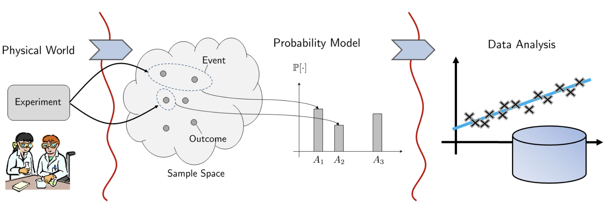
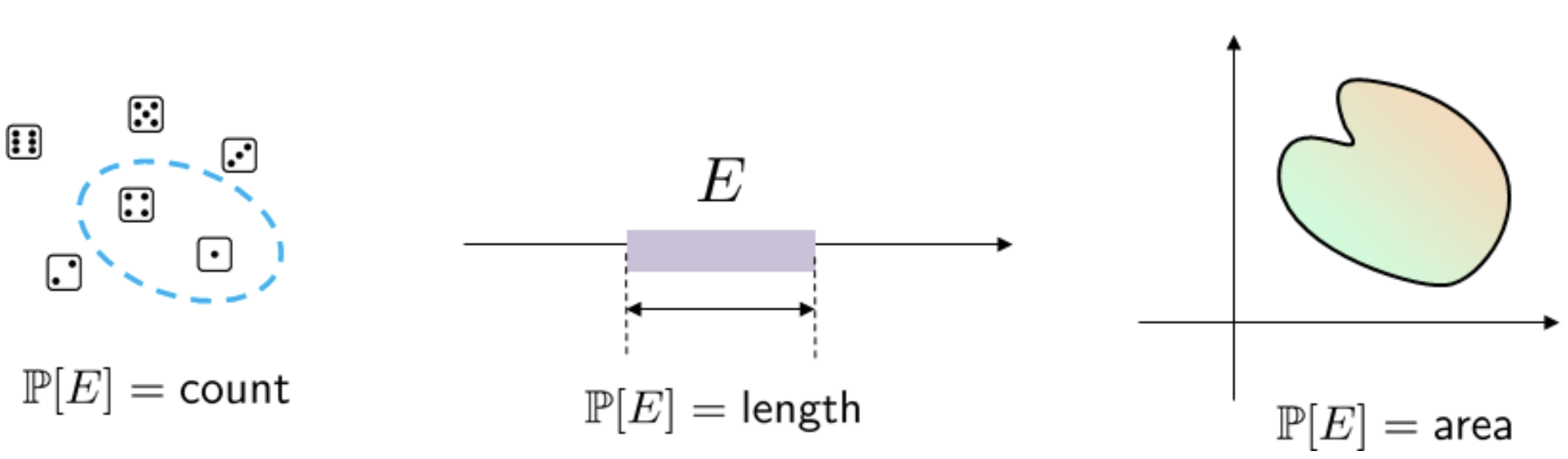
Probability is a measure of the size of a set of outcomes.
\text{Consistency: } E_1 \subseteq E_2 \;\Rightarrow\; \mathbb{P}(E_1) \leq \mathbb{P}(E_2).
Conditional Probability
What are possible values for the following probabilities: \begin{aligned} \mathbb{P}[\text{grass is wet} \mid \text{it rained}] \qquad & \mathbb{P}[\text{grass is wet}] \\ \mathbb{P}[\text{it rained} \mid \text{grass is wet}] \qquad & \mathbb{P}[\text{it rained}] \end{aligned}
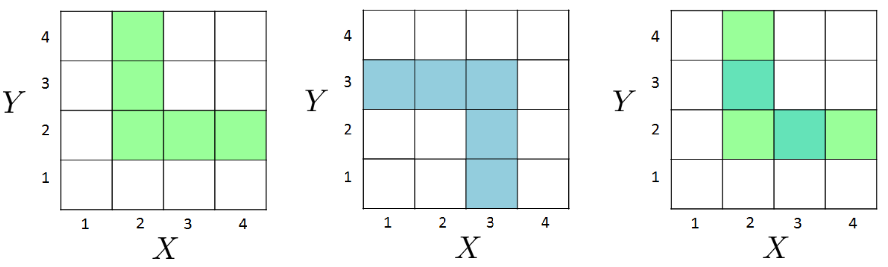
Consider a tetrahedral (4-sided) die. Let X be the first roll and Y be the second roll. Let B be the event that \min(X,Y)=2 and M be the event that \max(X,Y)=3. Find \mathbb{P}[M \mid B].
Bayes’ Theorem
🎥 3Blue1Brown — Bayes’ theorem visualized. Directly follows the lecture derivation.
🎥 3Blue1Brown — A concise visual proof of Bayes’ theorem (4 min).
🎥 3Blue1Brown — The medical test paradox: conditional probability in practice, with Bayes factors.
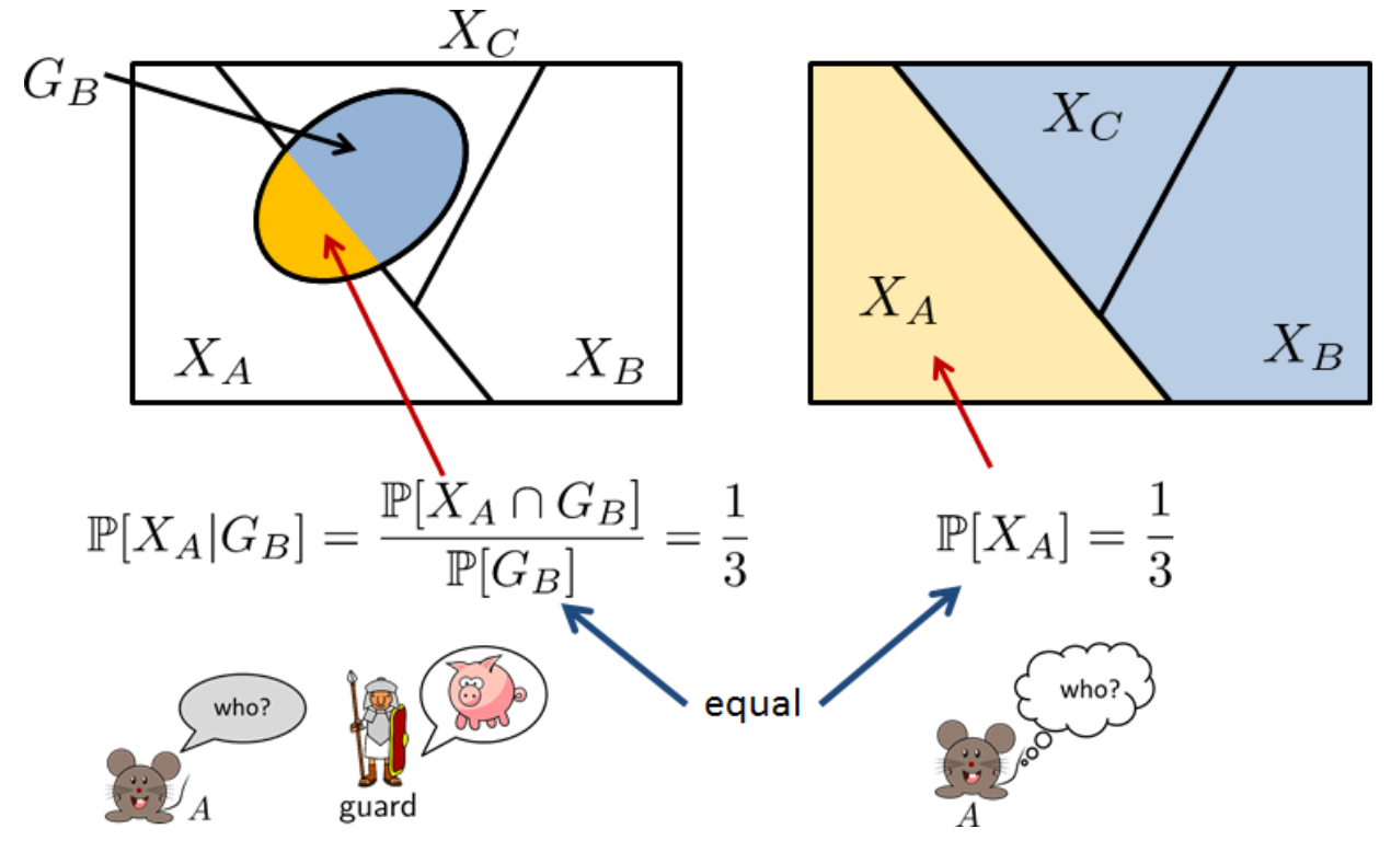
The king says that he will pardon two prisoners and sentence one.
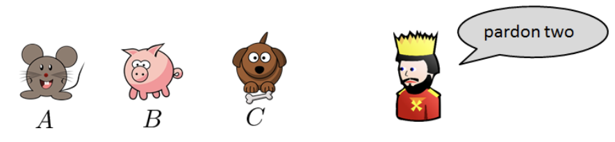
A friendly guard is allowed to tell prisoner A that prisoner B or prisoner C would be pardoned.
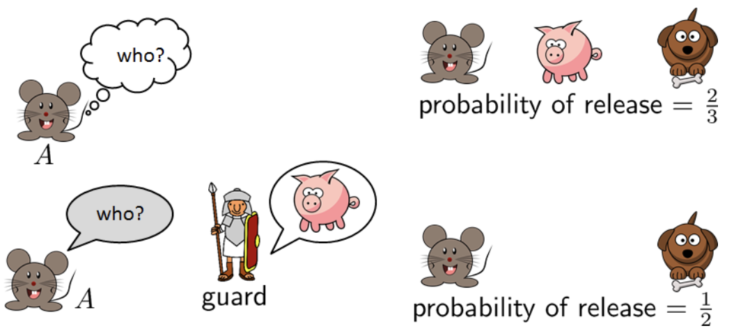
Should the prisoner ask or not ask?
Show answer image
Excursion: Bayesian Reasoning (see Jaynes)
Aristotelian logic based on syllogism, e.g.,
A \Rightarrow B \quad (\text{``A implies B''})
does not allow inversion, i.e., B \nRightarrow A.
In Bayesian reasoning, however, we have
A \Rightarrow B \;\;\Rightarrow\;\; \mathbb{P}(B \mid A) = 1
Because of Bayes’ rule,
\mathbb{P}(A \mid B) = \frac{\mathbb{P}(A)}{\mathbb{P}(B)} \ge \mathbb{P}(A)
“A becomes more likely when B is observed.”
Excursion: Bertrand’s Paradox
§ 2.2 Random Variables, Distributions and Densities
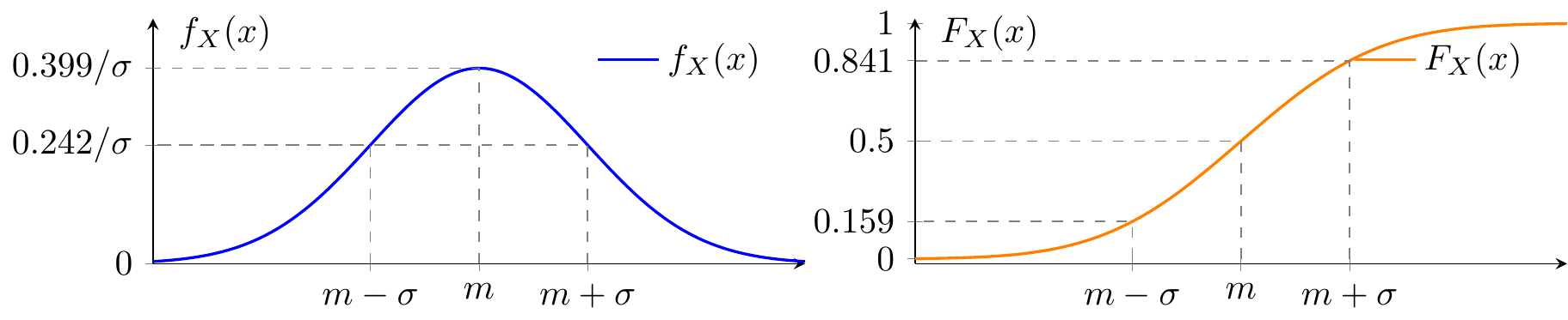
Cumulative Distribution Function and PDF
PDF & CDF explorer for 12 common distributions (Normal, Laplace, Rayleigh, Exponential, Cauchy, Binomial, Geometric, Poisson, Gamma, Erlang, Chi-square, Uniform) with adjustable parameters.
Joint and Conditional Distributions
Condition a 2D joint distribution on one variable and observe the resulting conditional PDF.
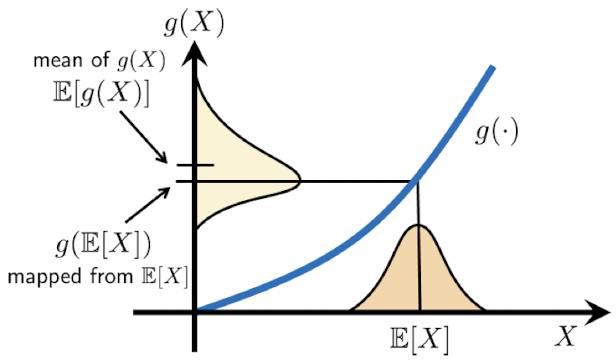
§ 2.3 Functions of Random Variables
Transformation of a Random Variable
The mapping Y = X^2, can be approximated by a piecewise linear mapping. 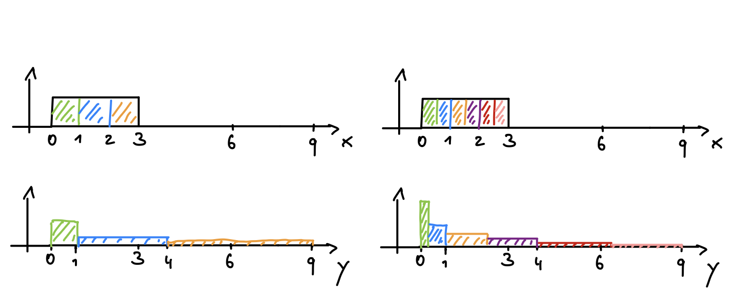
Probability distributions can be directly mapped. 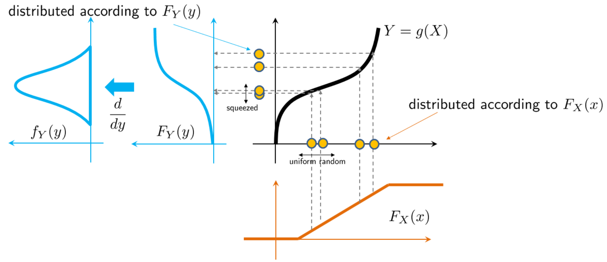
Apply a nonlinear transformation Y = g(X) to a chosen input distribution and watch the output PDF change in real time.
🎥 3Blue1Brown — Change of variables and the transformation formula for PDFs.
Mapping of Two Random Variables — Convolutions
🎥 3Blue1Brown — Why Gaussian + Gaussian = Gaussian: a visual proof via convolution.
§ 2.4 Expectations
Expectation Operator
St. Petersburg Paradox
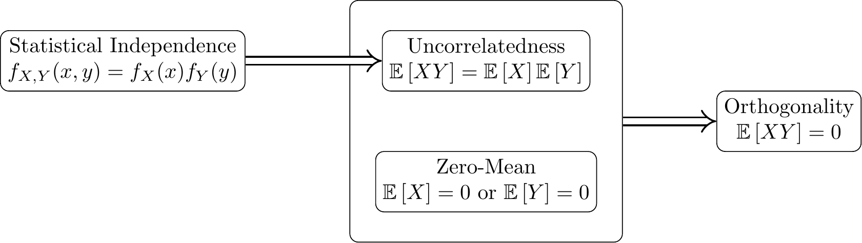
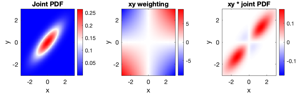
Correlation and Covariance
§ 2.5 Special Distributions
Distribution Explorer
Compare all major distributions in one place. Adjust parameters and switch between PDF and CDF view.
Binomial and Geometric Distributions
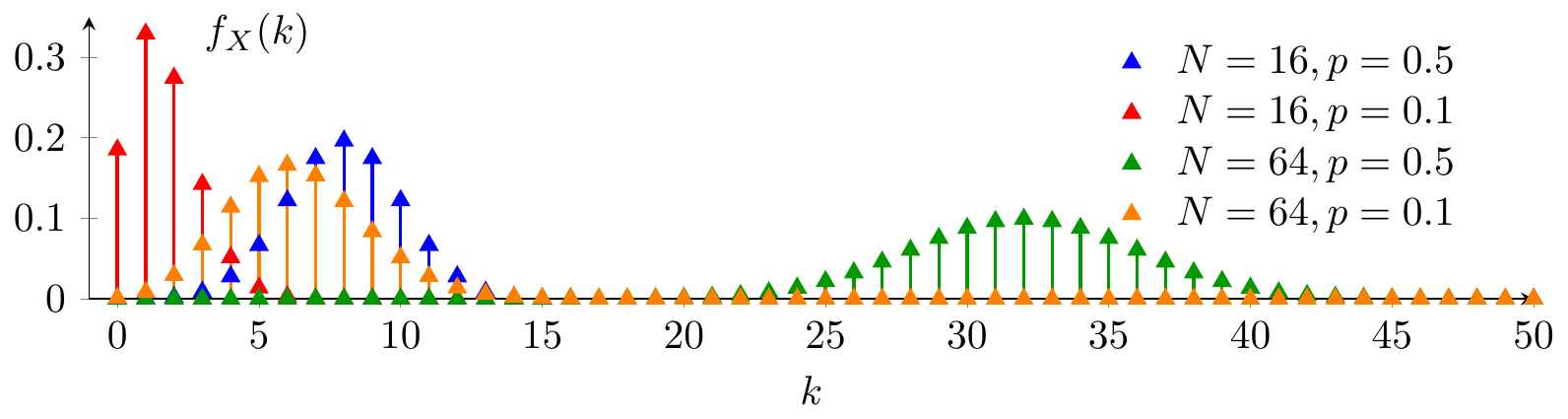
🎥 3Blue1Brown — Visualizing the binomial distribution and its Gaussian limit.
Excursion: Binomial Coefficient and Polynomials
Binomial coefficients arise when expanding powers of sums: (x+y)^n=\sum_{k=0}^n\binom{n}{k}x^k y^{\,n-k}.
This expansion can be understood combinatorially. Each term corresponds to choosing, for each of the n factors, either x or y. Thus, (x+y)^n enumerates all possible sequences of length n consisting of x and y.
For example, \begin{aligned} (x+y)^3 =\;& xxx + xxy + xyx + xyy \\ &+ yxx + yxy + yyx + yyy. \end{aligned}
Each term contains a certain number k of x’s and n-k of y’s. The binomial coefficient \binom{n}{k} counts how many such sequences exist, i.e., how many ways we can choose the positions of the x’s among the n factors.
Excursion: ABRACADABRA theorem
The ABRACADABRA theorem provides a surprising application of geometric distributions and martingales:
🎥 Numberphile — Expected waiting time to see ABRACADABRA in a random sequence.
Gaussian (Normal) Distribution
🎥 3Blue1Brown — Why \pi appears in the Gaussian PDF: the Herschel-Maxwell derivation.
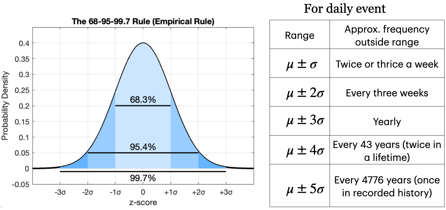
Excursion: Tails of the Gaussian
For Gaussian-distributed variables, the likelihood of an event is determined by its deviation from the mean, measured in standard deviations. The probabilities of falling within 1, 2, and 3 standard deviations are approximately 68%, 95%, and 99.7%, respectively, as described by the 68-95-99.7 rule.
Poisson Distribution
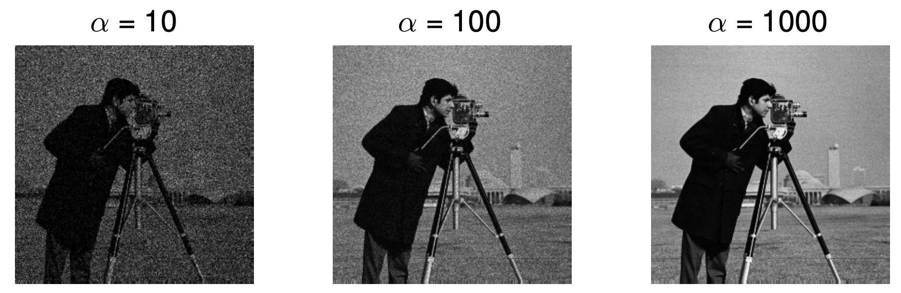
Photons arriving at an image sensor can be modeled as a Poisson process, where the arrival rate depends on the scene brightness.
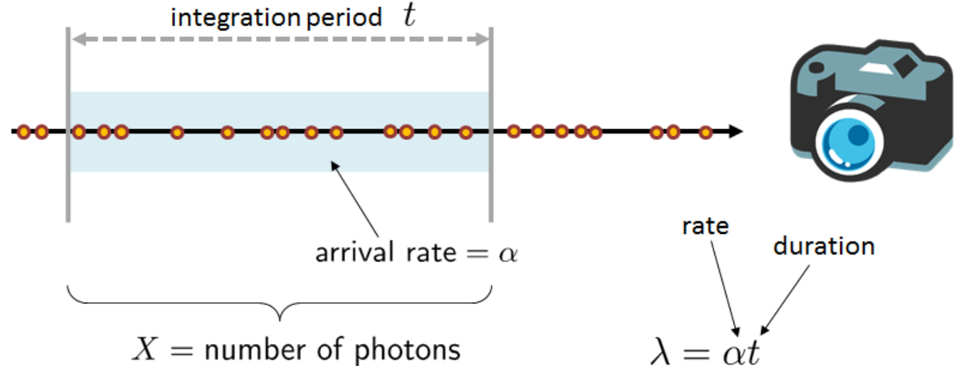
Random fluctuations in the image are called shot noise. The stronger the signal (\lambda), the higher the variance. However, the signal-to-noise ratio (SNR) still increases:
\mathrm{SNR} = \frac{\mathbb{E}[Y]}{\sqrt{\mathrm{Var}(Y)}} = \frac{\lambda}{\sqrt{\lambda}} = \sqrt{\lambda}.
Exponential Distribution
In a Poisson process, the number of arrivals in a fixed time interval follows a Poisson distribution, while the inter-arrival times are exponentially distributed. 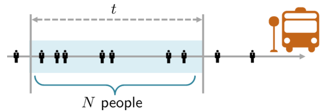

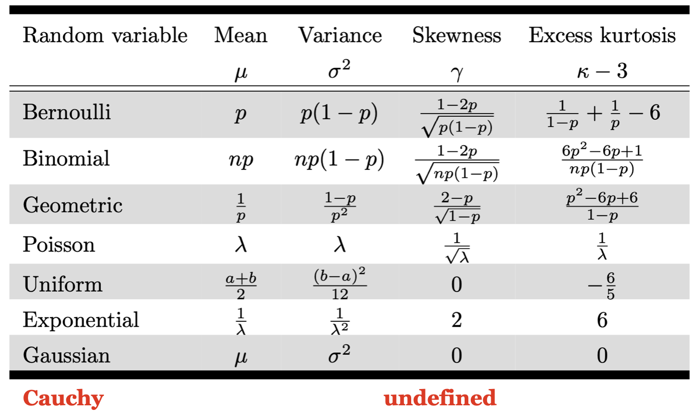
Moments Overview
§ 2.6 Limit Considerations
Jensen’s Inequality
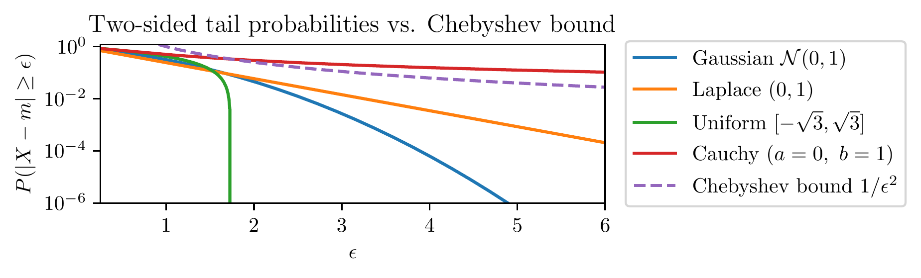
Markov and Chebyshev Inequalities
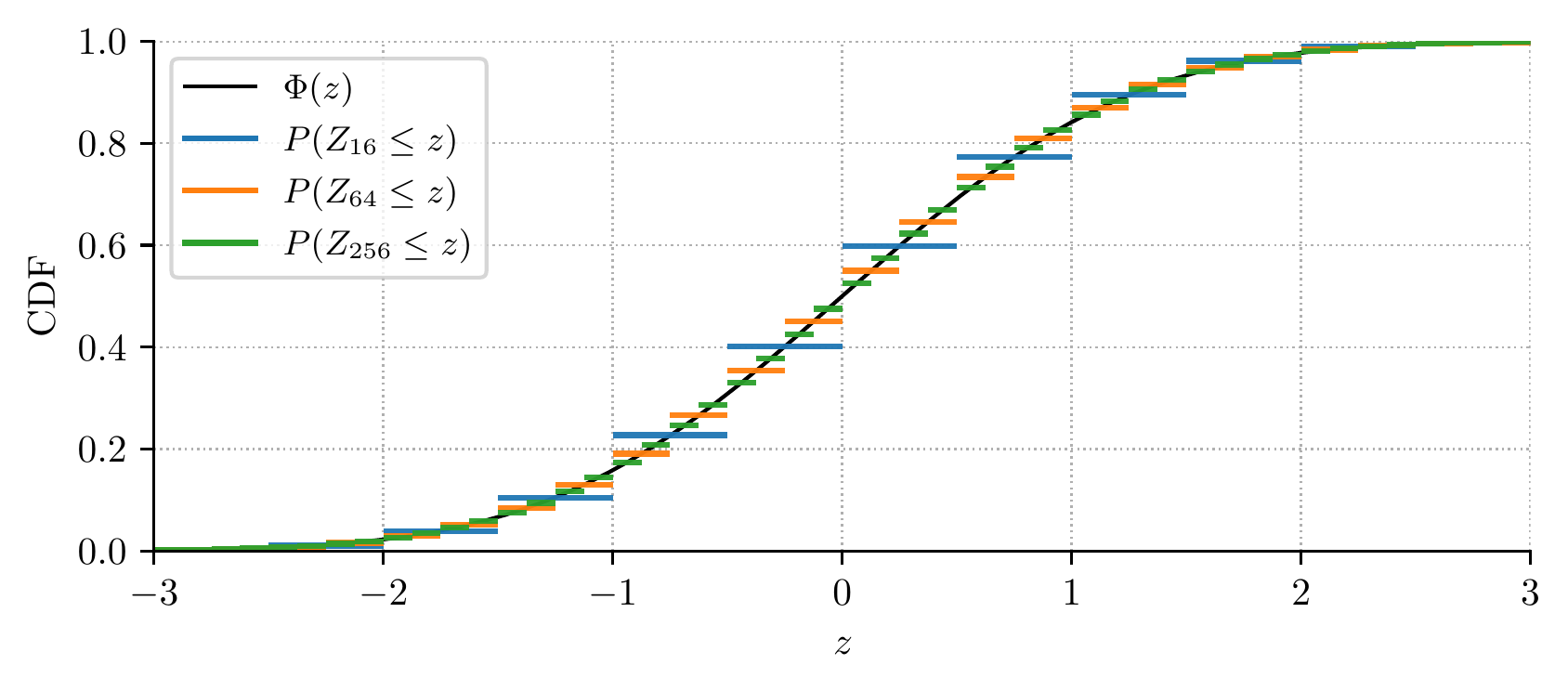
Central Limit Theorem
Animated convolution: add IID random variables one by one and watch the normalized sum converge to a Gaussian — for Laplace, Uniform, Rayleigh, Exponential, or Gamma source distributions.
🎥 3Blue1Brown — Why sample means converge to a normal distribution: a visual derivation (31 min).
§ 2.7 Jointly Distributed Random Variables
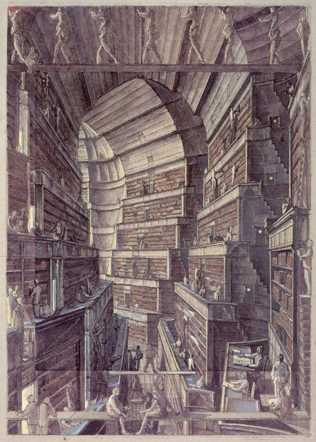
Excursion: The Library of Babel
The short story The Library of Babel by Jorge Luis Borges (1941) describes a library containing all possible books of length N, written using 25 basic characters (22 letters, the period, the comma, and the space).
This corresponds to the sample space of all sequences of length N over a finite alphabet \mathcal{A}, i.e., \Omega = \mathcal{A}^N, which underlies a multivariate (or product) distribution.
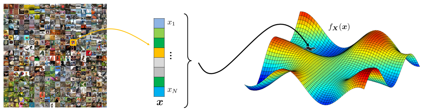
Excursion: ImageNet
One of the central datasets in modern deep learning is ImageNet. Images are typically resized to 224 \times 224 pixels with 3 color channels. When vectorized, this corresponds to \mathbf{x} \in \mathbb{R}^{150{,}528}.
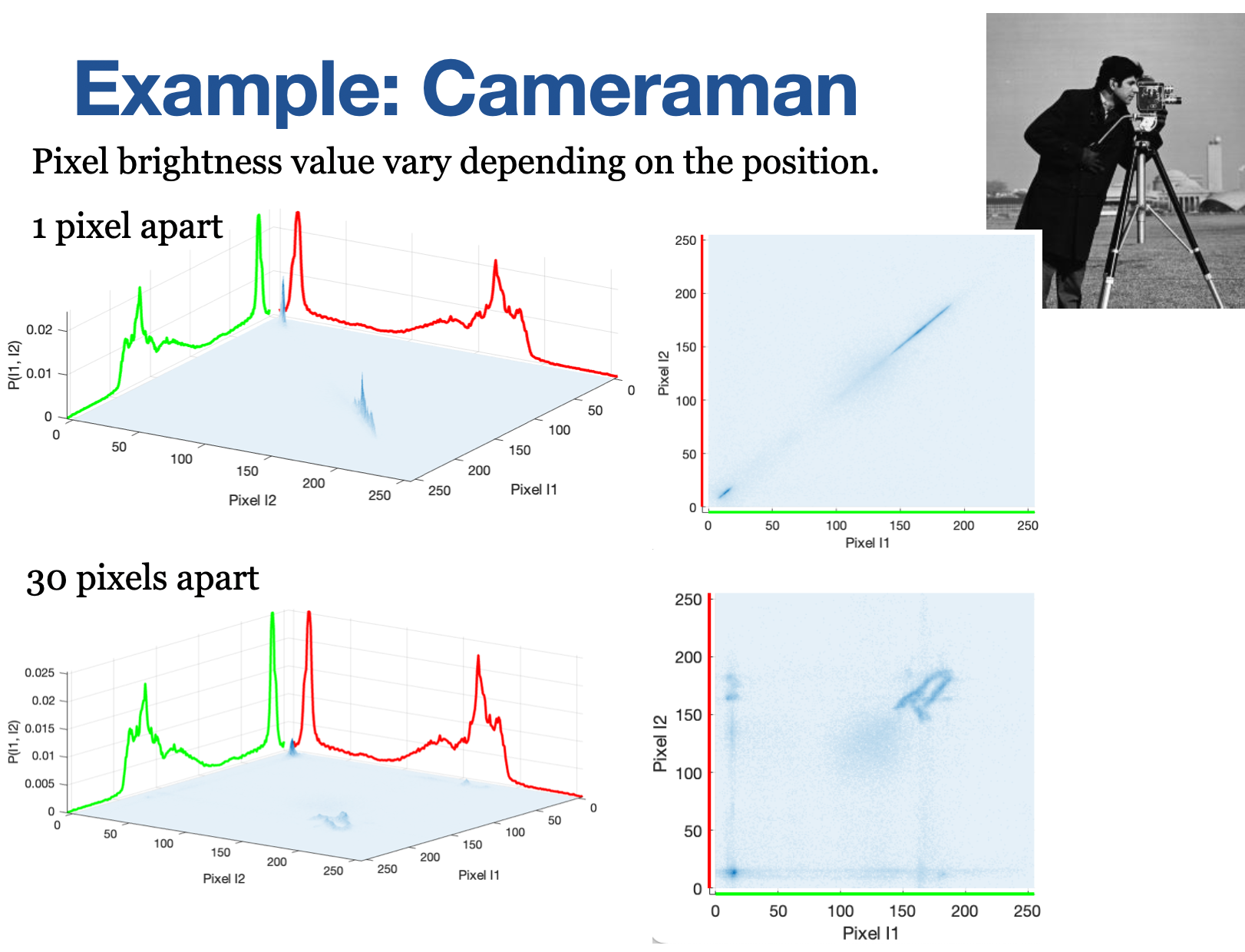
Spatial Distance and Joint Distribution
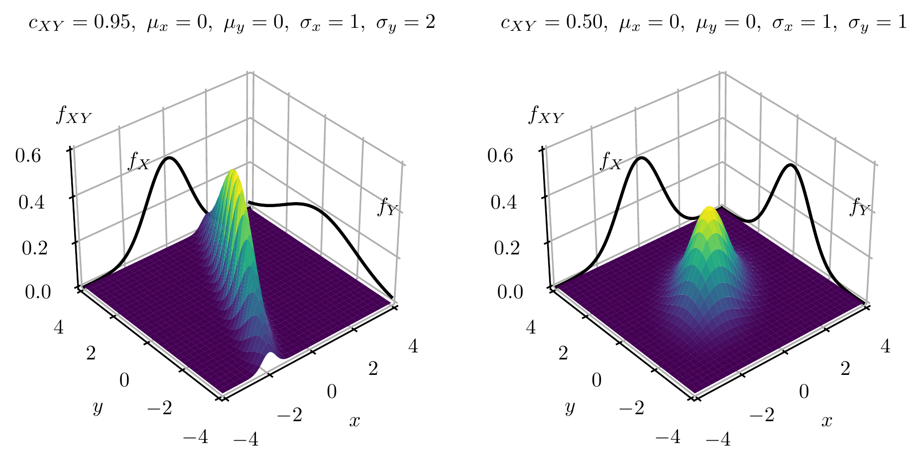
Multivariate Gaussian Distribution
Interactive 3D visualization of the bivariate Gaussian with adjustable means \mu_1, \mu_2, standard deviations \sigma_1, \sigma_2, and correlation coefficient \rho.
Visualizing Correlation
Joint PMF
The pairs of letters (for example in English texts) can be used to characterize the language. The letter pair in is the most common. 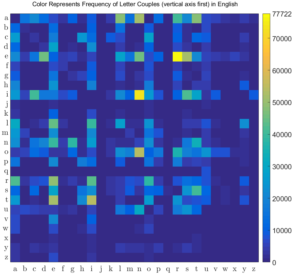
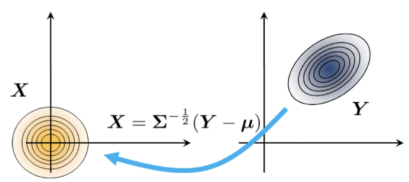
Transformation of Gaussians
![]()
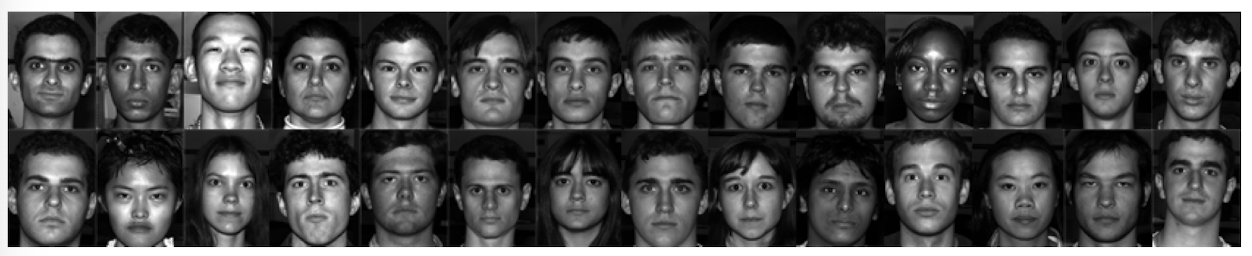
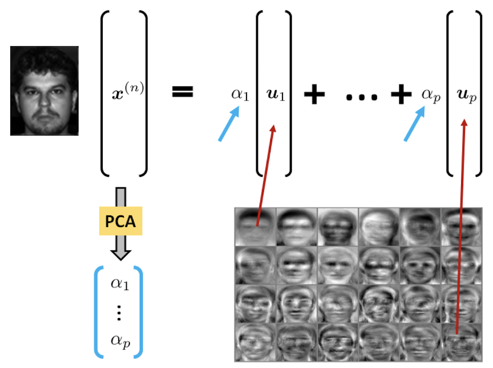
Excursion: Eigenfaces
Excursion: Properties and Surprising Behavior
🎥 “How We’re Fooled By Statistics” — regression to the mean in real-world data.