Practice Quizzes
Multiple-choice practice questions for all chapters. Each question may have more than one correct answer — select all that apply.
Ch 1 — Introduction
§ 1.1 Why This Course?
Q001 Randomness, Uncertainty, and Information
Probing the fundamental concepts of randomness, pseudo-randomness, and the role of uncertainty in information transmission
Which of the following statements about randomness and information in engineering are correct?
Consider the perspective of stochastic processes: the role of uncertainty, pseudo-randomness, and the relationship between randomness and information.
- In engineering, randomness is best understood as reflecting the observer’s uncertainty rather than an intrinsic property of the phenomenon
- A pseudo-random number generator produces truly random outputs since no observer can predict them
- Only stochastic signals can carry information
- A completely deterministic and predictable signal carries maximum information because it can be perfectly reconstructed
- If the exact initial conditions of a die throw were known, the outcome could in principle be predicted deterministically
- ✓ Correct. The course defines randomness as epistemic uncertainty — it reflects the observer’s limited knowledge, not necessarily a truly random mechanism.
- ✗ Incorrect. Pseudo-random generators are fully deterministic (completely determined by digital hardware or software); their outputs only appear random because the observer lacks knowledge of the internal state.
- ✓ Correct. As stated in the lecture: “Exclusively stochastic signals carry information.” A fully predictable signal conveys no new information — “no information without randomness.”
- ✗ Incorrect. Perfect predictability means zero surprise and therefore zero information content. Information is the “elimination of uncertainty” — without uncertainty, there is nothing to communicate.
- ✓ Correct. The die follows deterministic physical laws (Newton’s mechanics). The outcome is “random” only because the observer cannot know the initial conditions with sufficient precision.
Correct: The concept of randomness in this course is fundamentally tied to the observer’s knowledge. Randomness represents uncertainty, and information is the elimination of that uncertainty. This is why only stochastic (unpredictable) signals can carry information, and why even physically deterministic systems like dice can be modeled as random.
Review: Review the distinction between true randomness and pseudo-randomness, and consider why a fully predictable signal cannot carry information. Think about what “information” means from the receiver’s perspective: it is the elimination of uncertainty.
Ch 2 — Probability Theory
§ 2.1 Concept of Probability
Q002 Properties of Sample Spaces
Understanding the structure and classification of sample spaces in probability theory
Which of the following statements about sample spaces are correct?
Recall that the sample space H is the set of all possible outcomes of a random experiment.
- The sample space of “rolling a fair die” can be defined as H = \{1,2,3,4,5,6\} or as H = \{\text{even}, \text{odd}\}, depending on the formulation of the experiment
- A sample space must always be finite
- For measuring a voltage U with infinite precision where U_{\min} \leq U \leq U_{\max}, the sample space is uncountably infinite
- The sample space H = \{1, 2, 3, \ldots\} for “number of trials until winning the lottery” is uncountably infinite
- Each execution of a random experiment can yield multiple outcomes simultaneously
- ✓ Correct. The sample space depends on how the random experiment is defined. Both are valid sample spaces for different formulations of a die-rolling experiment.
- ✗ Incorrect. Sample spaces can be finite, countably infinite (e.g., number of trials until a lottery win: H = \{1, 2, 3, \ldots\}), or uncountably infinite (e.g., measuring a continuous voltage).
- ✓ Correct. The set of all real numbers in a continuous interval is uncountably infinite, which is the appropriate sample space for a continuous measurement with infinite precision.
- ✗ Incorrect. This sample space is countably infinite — the outcomes can be put into one-to-one correspondence with the natural numbers, even though the set is infinite.
- ✗ Incorrect. By definition, each execution of a random experiment yields exactly one outcome from the sample space.
Correct: Sample spaces are the foundation of probability theory and can take different forms depending on the experiment: finite (die roll), countably infinite (counting trials), or uncountably infinite (continuous measurements). The choice of sample space depends on the formulation of the random experiment.
Review: Review the three types of sample spaces and their examples. Remember: countable means the elements can be listed (even if infinitely), uncountable means they form a continuous set. Also recall that each single trial produces exactly one outcome.
Q003 Field of Events (Sigma-Algebra)
Understanding the defining properties and consequences of the field of events
Which of the following statements about the field of events \mathcal{A} are correct?
Recall the three defining properties:
- H \in \mathcal{A}
- A \in \mathcal{A} \Rightarrow \overline{A} \in \mathcal{A}
- A_1, A_2, \ldots \in \mathcal{A} \Rightarrow \bigcup_\nu A_\nu \in \mathcal{A}
- The impossible event \emptyset is always an element of \mathcal{A}
- The set \mathcal{A} = \{\emptyset, H\} is a valid field of events for any sample space H
- Every subset of H must be an element of \mathcal{A}
- For a countable sample space where all elementary events are in \mathcal{A}, the field of events corresponds to the power set of H
- If A \in \mathcal{A} and B \in \mathcal{A}, then A \cap B \in \mathcal{A}
- ✓ Correct. Since H \in \mathcal{A} (property 1) and complements are closed (property 2), we have \overline{H} = \emptyset \in \mathcal{A}.
- ✓ Correct. This is the smallest possible sigma-algebra (trivial sigma-algebra). It satisfies all three properties: H \in \mathcal{A}; \overline{H} = \emptyset \in \mathcal{A} and \overline{\emptyset} = H \in \mathcal{A}; \emptyset \cup H = H \in \mathcal{A}.
- ✗ Incorrect. The field of events can be strictly smaller than the power set. For example, \mathcal{A} = \{\emptyset, H\} is a valid field of events that does not contain all subsets of H.
- ✓ Correct. When all singletons belong to \mathcal{A}, the closure under unions and complements forces every subset of H to be in \mathcal{A}, which is exactly the power set.
- ✓ Correct. By De Morgan’s law, A \cap B = \overline{\overline{A} \cup \overline{B}}. Since \overline{A}, \overline{B} \in \mathcal{A} (property 2), their union is in \mathcal{A} (property 3), and its complement is also in \mathcal{A} (property 2).
Correct: The field of events \mathcal{A} is a structured collection of subsets of H that is closed under complementation, countable unions, and (by De Morgan) intersections. It can range from the trivial algebra \{\emptyset, H\} to the full power set, and the impossible event is always included as the complement of H.
Review: Review the three defining properties of \mathcal{A} and how they interact. Pay special attention to what is required versus what is optional: not every subset needs to be in \mathcal{A}, but certain closure properties must hold.
Q004 Axioms of Probability
Distinguishing axioms from their consequences and understanding the role of probability measures
Which of the following statements about the Kolmogorov axioms of probability are correct?
The three axioms state:
- \mathbb{P}(A) \geq 0
- \mathbb{P}(H) = 1
- \mathbb{P}(A_\mu \cup A_\nu) = \mathbb{P}(A_\mu) + \mathbb{P}(A_\nu) if A_\mu, A_\nu are disjoint
- The additivity axiom \mathbb{P}(A \cup B) = \mathbb{P}(A) + \mathbb{P}(B) applies to any two events A and B
- The axioms state that \mathbb{P}(A) \geq 0, but the upper bound \mathbb{P}(A) \leq 1 is a consequence, not an axiom
- The axioms uniquely determine the probability of every event in a given experiment
- The probability measure \mathbb{P}(\cdot) cannot be directly determined by measurements; it is related to relative frequency via the Law of Large Numbers
- For N disjoint events partitioning H, the axioms give \mathbb{P}(A_\nu) = 1/N without any additional assumption
- ✗ Incorrect. The additivity axiom applies only when A and B are disjoint (mutually exclusive). For general events, the inclusion-exclusion formula gives \mathbb{P}(A \cup B) = \mathbb{P}(A) + \mathbb{P}(B) - \mathbb{P}(A \cap B).
- ✓ Correct. From \mathbb{P}(A) + \mathbb{P}(\overline{A}) = \mathbb{P}(H) = 1 and \mathbb{P}(\overline{A}) \geq 0, it follows that \mathbb{P}(A) \leq 1. So the upper bound is derived, not axiomatically stated.
- ✗ Incorrect. The axioms define the properties that any probability measure must satisfy, but they do not specify which particular probability values to assign. Additional information (symmetry, empirical data, etc.) is needed to assign concrete probabilities.
- ✓ Correct. As stated in the lecture, “The probability \mathbb{P}(A) cannot be determined by measurements.” The transition from empirical relative frequency to theoretical probability is captured by the (Weak) Law of Large Numbers.
- ✗ Incorrect. The result \mathbb{P}(A_\nu) = 1/N requires the additional assumption that all elementary events are equally likely (Laplace assumption). The axioms alone only require non-negativity, normalization, and additivity — they do not impose equal probabilities.
Correct: The Kolmogorov axioms provide the minimal framework for probability: non-negativity, normalization, and countable additivity for disjoint events. Many familiar results (like \mathbb{P}(A) \leq 1 or Laplace probabilities) are consequences or require additional assumptions, not axioms themselves.
Review: Carefully distinguish between what the axioms state versus what can be derived from them. Also note that the axioms do not tell you which probability to assign — that requires modeling assumptions.
Q005 Conditional Probability and Bayes’ Theorem
Testing conceptual understanding of conditional probability, the chain rule, and the theorem of total probability
Which of the following statements about conditional probability and Bayes’ theorem are correct?
- \mathbb{P}(B|A) = \mathbb{P}(A|B) always holds
- In Bayes’ theorem \mathbb{P}(A|B) = \frac{\mathbb{P}(B|A) \, \mathbb{P}(A)}{\mathbb{P}(B)}, the term \mathbb{P}(A) is called the prior probability and \mathbb{P}(A|B) is the posterior probability
- The chain rule for conditional probabilities states \mathbb{P}(A, B \,|\, C) = \mathbb{P}(A \,|\, B, C) \cdot \mathbb{P}(B \,|\, C)
- The theorem of total probability requires the conditioning events A_\nu to form a partition: they must be disjoint and cover the entire sample space
- The theorem of total probability requires the conditioning events to have overlapping (non-disjoint) regions
- ✗ Incorrect. In general \mathbb{P}(B|A) = \mathbb{P}(A \cap B)/\mathbb{P}(A) while \mathbb{P}(A|B) = \mathbb{P}(A \cap B)/\mathbb{P}(B). These are equal only in the special case when \mathbb{P}(A) = \mathbb{P}(B).
- ✓ Correct. \mathbb{P}(A) is our belief about A before observing B (prior), and \mathbb{P}(A|B) is the updated belief after observing B (posterior). \mathbb{P}(B|A) is the likelihood.
- ✓ Correct. This follows from applying the definition of conditional probability twice: \mathbb{P}(A,B|C) = \mathbb{P}(A \cap B \cap C)/\mathbb{P}(C).
- ✓ Correct. The theorem states \mathbb{P}(B) = \sum_\nu \mathbb{P}(B|A_\nu) \mathbb{P}(A_\nu), which requires \bigcup_\nu A_\nu = H and A_\nu \cap A_\mu = \emptyset for \nu \neq \mu.
- ✗ Incorrect. The opposite is true: the conditioning events must be disjoint (mutually exclusive) and exhaustive, i.e., they form a partition of the sample space H.
Correct: Conditional probability is asymmetric (\mathbb{P}(A|B) \neq \mathbb{P}(B|A) in general), Bayes’ theorem provides a principled way to update beliefs, and the total probability theorem decomposes marginal probabilities using a partition of the sample space.
Review: Review the definitions of conditional probability, Bayes’ theorem (prior, likelihood, posterior), and the requirements for the theorem of total probability. Pay attention to the asymmetry of conditioning.
Q006 Bayesian Updating on a Binary Channel
Applying Bayes’ theorem and total probability to a concrete communication scenario
Consider a binary channel where the source symbols occur with \mathbb{P}(X_0) = 0.6 and \mathbb{P}(X_1) = 0.4. The channel error probabilities are \mathbb{P}(Y_1|X_0) = 0.1 (a ‘0’ is received as ‘1’) and \mathbb{P}(Y_0|X_1) = 0.2 (a ‘1’ is received as ‘0’).
Which of the following statements are correct?
- The total probability of a transmission error is \mathbb{P}(\text{Error}) = 0.2 \cdot 0.4 + 0.1 \cdot 0.6 = 0.14
- After receiving a ‘0’, the posterior \mathbb{P}(X_0|Y_0) \approx 0.87 is higher than the prior \mathbb{P}(X_0) = 0.6, illustrating how the observation updates our belief
- The Bayesian update changes the prior probability itself, so after the observation \mathbb{P}(X_0) becomes 0.87
- If the channel were symmetric (\mathbb{P}(Y_1|X_0) = \mathbb{P}(Y_0|X_1)), the posterior would always equal the prior regardless of the observation
- Since \mathbb{P}(Y_0|X_0) = 0.9 > \mathbb{P}(Y_0|X_1) = 0.2, observing Y_0 provides no useful information about which symbol was sent
- ✓ Correct. By the total probability theorem, \mathbb{P}(\text{Error}) = \mathbb{P}(Y_0|X_1)\mathbb{P}(X_1) + \mathbb{P}(Y_1|X_0)\mathbb{P}(X_0) = 0.08 + 0.06 = 0.14.
- ✓ Correct. \mathbb{P}(X_0|Y_0) = \mathbb{P}(Y_0|X_0)\mathbb{P}(X_0)/\mathbb{P}(Y_0) = (0.9 \times 0.6)/0.62 \approx 0.87. Receiving ‘0’ reinforces our belief that ‘0’ was sent.
- ✗ Incorrect. The prior \mathbb{P}(X_0) = 0.6 does not change. What we compute is a new, different quantity — the posterior \mathbb{P}(X_0|Y_0) \approx 0.87 — which is conditioned on the observation.
- ✗ Incorrect. Channel symmetry alone does not make the posterior equal to the prior. For example, with \epsilon = 0.1 and \mathbb{P}(X_0) = 0.6, the posterior \mathbb{P}(X_0|Y_0) = (0.9 \cdot 0.6)/(0.9 \cdot 0.6 + 0.1 \cdot 0.4) \approx 0.93 \neq 0.6. Only a completely useless channel (\epsilon = 0.5) would leave beliefs unchanged.
- ✗ Incorrect. The large difference in likelihoods (0.9 vs. 0.2) means observing Y_0 is highly informative — it strongly favors X_0 over X_1, as reflected in the posterior rising from 0.6 to 0.87.
Correct: Bayes’ theorem allows us to update beliefs based on observations. The prior \mathbb{P}(X_0) is a property of the source; the posterior \mathbb{P}(X_0|Y_0) incorporates the observation. The total probability theorem is used to compute the evidence \mathbb{P}(Y_0) from the individual likelihoods and priors.
Review: Work through the binary channel example step by step. Compute \mathbb{P}(Y_0) using total probability, then apply Bayes’ theorem. Note that the prior is not modified — the posterior is a separate, conditional quantity.
Q007 Statistical Independence of Events
Understanding independence, its definition, and common misconceptions involving disjointness
Which of the following statements about statistical independence of events are correct?
- If A and B are independent, then \mathbb{P}(A \cap B) = \mathbb{P}(A) \cdot \mathbb{P}(B)
- If \mathbb{P}(A \cap B) = 0, then A and B must be independent
- If A and B are independent, then \mathbb{P}(A|B) = \mathbb{P}(A), meaning we cannot learn about A by observing B
- Independence of events is the same as events being disjoint (mutually exclusive)
- For three events A_1, A_2, A_3, pairwise independence is sufficient to guarantee mutual independence
- ✓ Correct. This is the definition of statistical independence for two events.
- ✗ Incorrect. \mathbb{P}(A \cap B) = 0 means the events are disjoint (mutually exclusive), not independent. In fact, if both \mathbb{P}(A) > 0 and \mathbb{P}(B) > 0, disjoint events are always dependent: knowing one occurred tells you the other did not.
- ✓ Correct. From the definition, \mathbb{P}(A|B) = \mathbb{P}(A \cap B)/\mathbb{P}(B) = \mathbb{P}(A)\mathbb{P}(B)/\mathbb{P}(B) = \mathbb{P}(A). The posterior equals the prior, so observing B provides no information about A.
- ✗ Incorrect. Independence (\mathbb{P}(A \cap B) = \mathbb{P}(A)\mathbb{P}(B)) and disjointness (A \cap B = \emptyset) are fundamentally different. Disjoint events with nonzero probabilities are always dependent since 0 = \mathbb{P}(A \cap B) \neq \mathbb{P}(A)\mathbb{P}(B) > 0.
- ✗ Incorrect. Pairwise independence does not imply mutual independence. Mutual independence additionally requires \mathbb{P}(A_1 \cap A_2 \cap A_3) = \mathbb{P}(A_1)\mathbb{P}(A_2)\mathbb{P}(A_3), which does not follow from the pairwise conditions alone.
Correct: Independence means that the joint probability factorizes into the product of marginals, and consequently one event provides no information about the other. This is very different from disjointness, where the events cannot co-occur.
Review: Carefully distinguish between independence (\mathbb{P}(A \cap B) = \mathbb{P}(A)\mathbb{P}(B)) and disjointness (A \cap B = \emptyset). Think about what each concept implies: can two disjoint events with positive probability be independent?
Q008 Combined Experiments and Product Events
Understanding Cartesian products of sample spaces and probabilities of product events
Consider combining two random experiments with sample spaces H_1 and H_2. Which of the following statements are correct?
- The sample space of the combined experiment is the Cartesian product H = H_1 \times H_2
- For the combined experiment “coin toss and die roll,” the sample space has 2 \times 6 = 12 elements
- If the individual experiments are independent, then \mathbb{P}(A \times B) = \mathbb{P}(A) \cdot \mathbb{P}(B) for events A \subseteq H_1 and B \subseteq H_2
- In the double coin toss experiment, ‘HT’ and ‘TH’ represent the same outcome since both contain one head and one tail
- The product event C = A \times B is a subset of the combined sample space H = H_1 \times H_2
- ✓ Correct. By definition, the combined sample space consists of all ordered pairs of outcomes from the individual experiments.
- ✓ Correct. H_1 = \{\text{H}, \text{T}\} has 2 elements, H_2 = \{1,2,3,4,5,6\} has 6 elements, so |H| = 12 with elements like ‘H1’, ‘H2’, …, ‘T6’.
- ✓ Correct. For independent product events, the joint probability factorizes into the product of the marginal probabilities.
- ✗ Incorrect. ‘HT’ and ‘TH’ are distinct outcomes — they differ in the order of sub-outcomes. Whether the same coin is tossed twice (different temporal order) or two different coins are tossed, the ordered pairs are distinguishable.
- ✓ Correct. Since A \subseteq H_1 and B \subseteq H_2, their Cartesian product satisfies A \times B \subseteq H_1 \times H_2 = H.
Correct: Combined experiments are modeled by Cartesian products of sample spaces. Product events inherit the product structure, and independence of the sub-experiments ensures that joint probabilities factorize. Remember that ordered pairs distinguish outcomes by position.
Review: Review how Cartesian products work and why ‘HT’ \neq ‘TH’ in the product space. The order within the pair matters because the two positions correspond to different sub-experiments.
Q009 Bernoulli Experiments
Understanding the Bernoulli formula and the combinatorial structure of repeated independent trials
A fair coin (p = 0.5) is tossed N = 10 times. Which of the following statements about this Bernoulli experiment are correct?
- The probability of getting exactly 3 heads is \binom{10}{3} \cdot 0.5^3 \cdot 0.5^7
- The probability of getting heads in three specific pre-determined trials (e.g., trials 1, 4, 7) and tails in all others is \binom{10}{3} \cdot 0.5^{10}
- The outcomes of all 10 trials are statistically independent of each other
- The probability of getting at least one head is 1 - 0.5^{10}
- The probability of getting exactly 5 heads is lower than the probability of getting exactly 3 heads, because 5 heads is a “more extreme” outcome
- ✓ Correct. By the Bernoulli formula, \mathbb{P}(\text{exactly } k \text{ successes in } N \text{ trials}) = \binom{N}{k} p^k (1-p)^{N-k}.
- ✗ Incorrect. For specific pre-determined trials, there is no combinatorial factor — the probability is simply 0.5^3 \cdot 0.5^7 = 0.5^{10} \approx 9.77 \times 10^{-4}. The binomial coefficient \binom{10}{3} counts the number of ways to choose which 3 trials have heads, which is not needed when the trials are already specified.
- ✓ Correct. By definition, Bernoulli experiments require that all individual trials are statistically independent.
- ✓ Correct. Using the complement: \mathbb{P}(\text{at least 1 head}) = 1 - \mathbb{P}(\text{no heads}) = 1 - (1-p)^N = 1 - 0.5^{10}.
- ✗ Incorrect. For a fair coin (p = 0.5), k = 5 (half of N = 10) is actually the most likely outcome. \binom{10}{5} = 252 > \binom{10}{3} = 120, so \mathbb{P}(k=5) > \mathbb{P}(k=3).
Correct: In a Bernoulli experiment, independence of trials is fundamental. The binomial coefficient \binom{N}{k} counts the number of distinct orderings and is needed only when we ask for exactly k successes in any trials, not in pre-specified ones. For a fair coin, the mode of the binomial distribution is at k = N/2.
Review: Review when the combinatorial factor \binom{N}{k} appears in the Bernoulli formula and when it does not. Also consider which value of k maximizes \binom{N}{k} for fixed N.
Q010 Law of Large Numbers and Bernoulli’s Theorem
Understanding the convergence of relative frequency to probability and the nature of probabilistic statements
Which of the following statements about the Weak Law of Large Numbers (WLLN) and Bernoulli’s Theorem are correct?
- The WLLN states that \lim_{N \to \infty} \mathbb{P}\!\left(|\mathbb{P}(A) - h_N(A)| \leq \epsilon\right) = 1 for any \epsilon > 0
- Bernoulli’s Theorem states that the bound on the deviation probability is \mathbb{P}\!\left(|k/N - p| > \epsilon\right) < p(1-p)/(N\epsilon^2), which is tightest (smallest) when p = 0.5
- The relative frequency h_N(A) = n_A / N is itself a random variable
- The WLLN implies that after sufficiently many trials, the relative frequency will never deviate from the true probability
- Bernoulli’s Theorem applies to any sequence of trials, regardless of whether they are independent
- ✓ Correct. This is the precise statement of the Weak Law of Large Numbers, expressing convergence in probability of the relative frequency h_N(A) to the true probability \mathbb{P}(A).
- ✗ Incorrect. The factor p(1-p) is maximized at p = 0.5 (where it equals 0.25), making the bound loosest (largest). The bound is tightest when p is near 0 or 1.
- ✓ Correct. Since h_N(A) depends on the random outcomes of N trials, it is a random variable. Its randomness is precisely what makes the WLLN a probabilistic (not deterministic) convergence statement.
- ✗ Incorrect. The WLLN is a statement about probabilities, not certainties. For any finite N, there is always a nonzero probability of deviation. Even for large N, deviations are theoretically possible — they are just increasingly unlikely.
- ✗ Incorrect. Bernoulli’s Theorem specifically applies to Bernoulli experiments, where all trials are statistically independent and the probability of the event is the same in each trial.
Correct: The WLLN and Bernoulli’s Theorem provide the bridge between the theoretical concept of probability and empirical relative frequency. The convergence is probabilistic — not deterministic — and the relative frequency itself is a random variable whose variability decreases with more trials.
Review: Review the precise statement of the WLLN (convergence in probability, not certainty) and the conditions under which Bernoulli’s Theorem applies (independent, identically distributed trials). Also examine how the bound p(1-p)/(N\epsilon^2) behaves as a function of p.
§ 2.2 Random Variables, Distributions and Densities
Q011 Definition of Random Variables
Understanding what a random variable is and how it relates to the sample space
Which of the following statements about random variables (RVs) are correct?
- A random variable is a mapping from the sample space H to the real numbers: X: H \mapsto \mathbb{R}
- The value x_i = X(\eta_i) assigned to a specific outcome \eta_i is called a realization of the RV X
- A random variable is itself a random number
- On a given sample space, only one random variable can be defined
- A complex-valued RV Z(\eta) = X(\eta) + jY(\eta) combines two real-valued RVs that depend on the same outcome \eta
- ✓ Correct. By definition, a real-valued random variable assigns a real number to each outcome \eta_i of a random experiment.
- ✓ Correct. A realization is the concrete numerical value that the RV takes for a particular outcome.
- ✗ Incorrect. A random variable is a function (a mapping), not a number. It maps outcomes from the sample space to real numbers. The randomness arises because the outcome \eta of the experiment is uncertain.
- ✗ Incorrect. Multiple different random variables can be defined on the same sample space. For example, for a die roll, one RV could map outcomes to \{10, 20, \ldots, 60\} while another maps them to \{-1, +1\} based on parity.
- ✓ Correct. A complex RV is decomposed into real and imaginary parts, both of which are real-valued RVs defined on the same sample space and depending on the same outcome.
Correct: A random variable is fundamentally a function — a deterministic mapping from outcomes to numbers. The “randomness” comes entirely from the uncertainty about which outcome \eta occurs. Multiple RVs can coexist on the same sample space, providing different numerical views of the same experiment.
Review: Revisit the formal definition: X: H \mapsto \mathbb{R}. A random variable is a function, not a number. Think about the die roll examples where different RVs assign different numbers to the same outcomes.
Q012 Properties of the CDF
Understanding the cumulative distribution function and its fundamental properties
Which of the following statements about the cumulative distribution function (CDF) F_X(x) = \mathbb{P}(X \leq x) are correct?
- F_X(x) is monotonically increasing, meaning F_X(x_2) \geq F_X(x_1) whenever x_2 > x_1
- F_X(-\infty) = 0 and F_X(\infty) = 1
- The probability \mathbb{P}(x_1 < X \leq x_2) can be computed as F_X(x_2) - F_X(x_1)
- The CDF can take negative values when the RV itself takes negative values
- The CDF of a discrete RV is a smooth, differentiable curve
- ✓ Correct. Since \{X \leq x_1\} \subseteq \{X \leq x_2\} for x_2 > x_1, the probability can only increase or stay the same.
- ✓ Correct. The probability that the RV takes a value less than -\infty is zero (impossible event), and the probability that it takes any finite value is one (certain event).
- ✓ Correct. This follows directly from \mathbb{P}(x_1 < X \leq x_2) = \mathbb{P}(X \leq x_2) - \mathbb{P}(X \leq x_1) = F_X(x_2) - F_X(x_1).
- ✗ Incorrect. The CDF is a probability and therefore always satisfies 0 \leq F_X(x) \leq 1, regardless of whether the RV takes negative values. The sign of x does not affect the range of F_X.
- ✗ Incorrect. For a discrete RV, the CDF is a step function with jumps at each possible value. The step heights correspond to the probabilities of the respective values. It is not differentiable at the jump points (in the classical sense).
Correct: The CDF has three fundamental properties: it is bounded between 0 and 1, it is monotonically non-decreasing, and its boundary values are F_X(-\infty) = 0 and F_X(\infty) = 1. Differences of CDF values give probabilities of intervals.
Review: Remember that the CDF is a probability, so its range is [0,1] — the values of the RV do not affect this. Also recall how discrete RVs produce step-function CDFs.
Q013 Properties of the PDF
Understanding the probability density function and its relationship to probability
Which of the following statements about the probability density function (PDF) f_X(x) = \frac{dF_X(x)}{dx} are correct?
- The PDF satisfies f_X(x) \leq 1 for all x, since it represents a probability
- \int_{-\infty}^{\infty} f_X(x) \, dx = 1
- For a continuous RV, the probability of taking an exact value x_0 is \mathbb{P}(X = x_0) = f_X(x_0)
- f_X(x) \geq 0 for all x
- The PDF of a discrete RV with values x_i and probabilities \mathbb{P}(x_i) is f_X(x) = \sum_i \mathbb{P}(x_i) \cdot \delta(x - x_i)
- ✗ Incorrect. The PDF is not a probability — it is a density. Values f_X(x) > 1 are perfectly possible, for example when a continuous RV is concentrated in a narrow interval.
- ✓ Correct. This normalization condition follows from F_X(\infty) = 1 and the fundamental theorem of calculus.
- ✗ Incorrect. For a continuous RV, \mathbb{P}(X = x_0) = 0 always. The PDF gives probability only through integration over an interval, not at a single point. Only for discrete RVs (via Dirac impulses) does a point mass exist.
- ✓ Correct. Since the CDF F_X(x) is monotonically increasing, its derivative (the PDF) is non-negative everywhere.
- ✓ Correct. Differentiating the step-function CDF produces Dirac delta impulses at each possible value, with weights equal to the corresponding probabilities.
Correct: The PDF is a density, not a probability itself. It can exceed 1 and gives probabilities only through integration. For continuous RVs, point probabilities are always zero. For discrete RVs, the PDF is a sum of weighted Dirac impulses.
Review: Carefully distinguish between a density and a probability. The PDF f_X(x) at a point is not the probability of that point — probability is obtained by integrating the PDF over an interval. Review the discrete case where Dirac impulses arise.
Q014 Discrete vs Continuous Random Variables
Recognizing the fundamental differences between discrete and continuous RVs in their CDF and PDF representations
Consider the CDF and PDF of a discrete RV (die roll, top) and a continuous RV (distance in unit square, bottom) shown below.
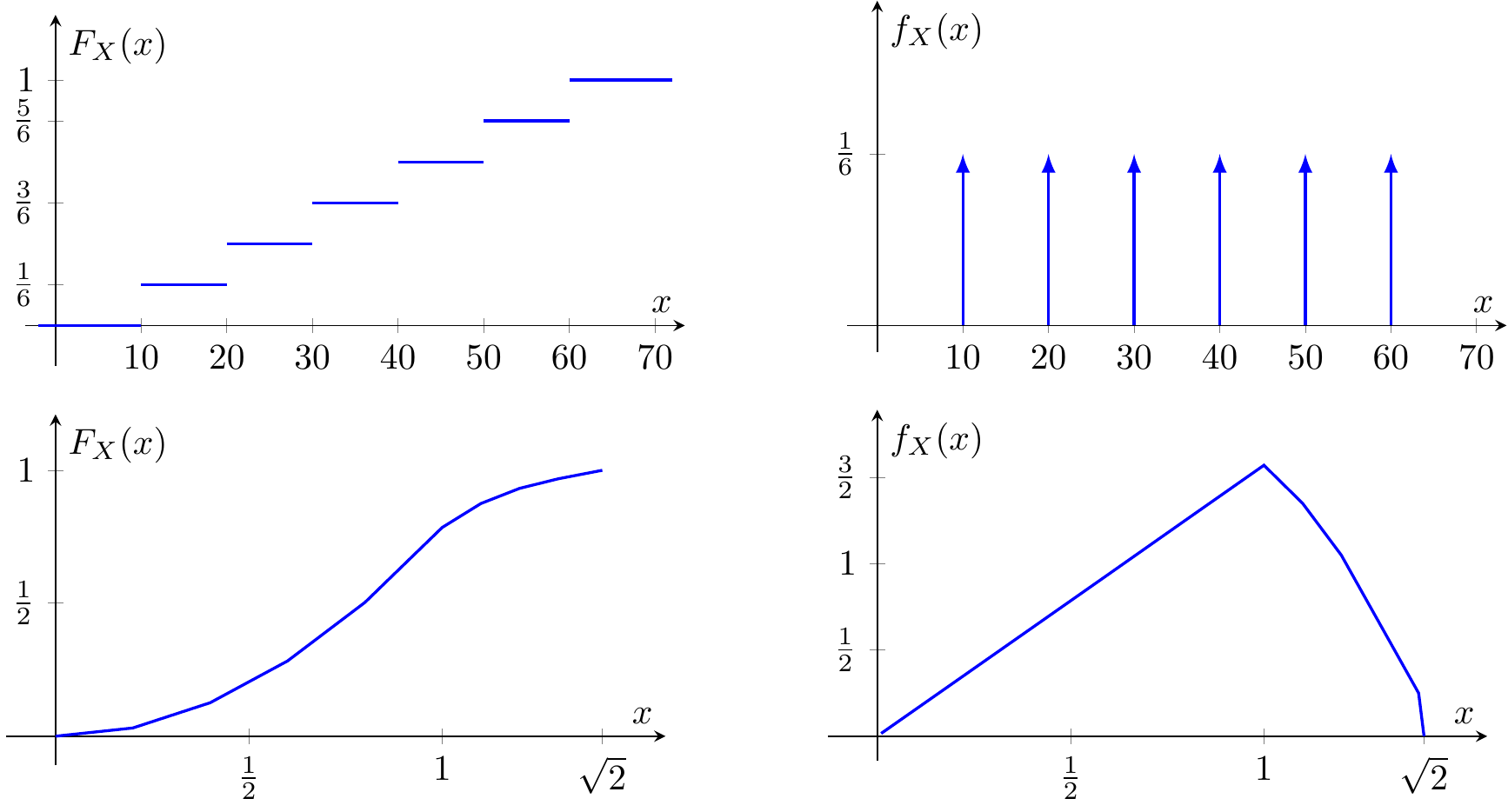
Which of the following statements are correct?
- For the discrete RV, each step in the CDF corresponds to a Dirac impulse in the PDF whose weight equals the step height
- For the continuous RV, \mathbb{P}(X = 1.0) = 0 even though f_X(1.0) > 0
- The CDF of the discrete RV is a continuous curve that smoothly increases from 0 to 1
- The area under the PDF curve is 1 for the continuous RV but not necessarily 1 for the discrete RV
- For the die roll with outcomes \{10, 20, 30, 40, 50, 60\} and equal probabilities, each Dirac impulse in the PDF has weight 1/6
- ✓ Correct. Differentiating a step function produces Dirac delta functions at the jump locations, with amplitudes equal to the step heights (probabilities).
- ✓ Correct. For continuous RVs, the probability of any single point is always zero. The PDF value f_X(x) > 0 indicates density, not probability — probability is obtained only by integrating over an interval.
- ✗ Incorrect. The CDF of a discrete RV is a step function with discontinuous jumps at each possible value. Between jumps, the CDF is flat (constant).
- ✗ Incorrect. The total “area” (integral) under the PDF is always 1, for both discrete and continuous RVs. For discrete RVs, the Dirac impulses have weights that sum to 1, satisfying \int f_X(x) \, dx = \sum_i \mathbb{P}(x_i) = 1.
- ✓ Correct. A fair die assigns equal probability 1/6 to each outcome, so f_X(x) = \frac{1}{6}\sum_{i=1}^{6}\delta(x - 10i).
Correct: Discrete RVs have step-function CDFs and Dirac-impulse PDFs. Continuous RVs have smooth CDFs and integrable PDFs. In both cases, the total integral of the PDF equals 1, and for continuous RVs, point probabilities are zero even where the density is positive.
Review: Review the relationship between CDF steps and PDF Dirac impulses for discrete RVs. Remember that the normalization \int f_X(x) \, dx = 1 holds universally.
Q015 Quantiles and Median
Understanding quantiles, percentiles, and the median as descriptors of a distribution
Which of the following statements about quantiles and the median are correct?
The n-th q-quantile of X is the smallest value x_u with u = n/q such that F_X(x_u) \geq u.
- The median is the value x_{0.5} such that F_X(x_{0.5}) \geq 0.5, i.e., at least half the probability mass lies at or below the median
- The 90th percentile x_{0.9} is the value below which 90% of the probability mass lies
- The median of a symmetric distribution always equals the mean
- For a discrete RV like a fair die with outcomes \{10, 20, 30, 40, 50, 60\}, the median is x_{0.5} = 35
- Quartiles divide the distribution into four parts of equal probability (25% each)
- ✓ Correct. The median is the first 2-quantile (q = 2, n = 1, u = 0.5), dividing the distribution so that at least 50% of the probability is at or below x_{0.5}.
- ✓ Correct. Percentiles are 100-quantiles, so the 90th percentile satisfies F_X(x_{0.9}) \geq 0.9.
- ✗ Incorrect in general. While this is true for symmetric distributions that have a finite mean (e.g., Gaussian), some symmetric distributions like the Cauchy distribution have no finite mean at all. The median exists for any distribution, but the mean need not.
- ✗ Incorrect. The median is the smallest value x such that F_X(x) \geq 0.5. Since F_X(30) = 3/6 = 0.5 \geq 0.5, the median is x_{0.5} = 30, not 35. For discrete RVs, the median must be one of the possible values.
- ✗ Incorrect in general. For continuous distributions this is true, but for discrete distributions, exact 25% splits may not be achievable. Quartiles are defined as the smallest values satisfying F_X(x_u) \geq u for u \in \{0.25, 0.5, 0.75\}, which may not produce exactly equal-sized groups.
Correct: Quantiles provide a robust way to describe the spread of a distribution. The median is the central quantile (u = 0.5), and percentiles divide the distribution into 100 parts. For discrete distributions, quantiles must snap to actual possible values.
Review: Review the formal definition of quantiles as the smallest value where F_X(x_u) \geq u. For discrete RVs, this means the quantile is always one of the possible values, not an interpolated number.
Q016 Uniform Distribution
Properties of uniformly distributed random variables (discrete and continuous)
Which of the following statements about the uniform distribution are correct?
- For a continuous uniform RV on [x_{\min}, x_{\max}], the PDF is f_X(x) = \frac{1}{x_{\max} - x_{\min}} within the interval and zero outside
- The CDF of a continuous uniform RV on [x_{\min}, x_{\max}] is a straight line with slope \frac{1}{x_{\max} - x_{\min}} within the interval
- For a uniformly distributed discrete RV with N possible values, the PDF is f_X(x) = \frac{1}{N} \sum_{i=1}^{N} \delta(x - x_i)
- A continuous uniform RV on [0, 1] satisfies \mathbb{P}(0.2 < X \leq 0.5) = 0.3
- For a continuous uniform RV on [0, 2], we have f_X(1) = 1 and therefore \mathbb{P}(X = 1) = 1
- ✓ Correct. The uniform density is constant over [x_{\min}, x_{\max}] and zero elsewhere, with height chosen so the total area equals 1.
- ✓ Correct. Integrating the constant PDF gives F_X(x) = \frac{x - x_{\min}}{x_{\max} - x_{\min}} for x \in [x_{\min}, x_{\max}], which is linear.
- ✓ Correct. Each value has equal probability 1/N, represented by equally weighted Dirac impulses.
- ✓ Correct. \mathbb{P}(0.2 < X \leq 0.5) = F_X(0.5) - F_X(0.2) = 0.5 - 0.2 = 0.3 for a uniform RV on [0,1].
- ✗ Incorrect. While f_X(1) = 1/(2-0) = 0.5 (not 1), even if the PDF value were 1, this would not imply \mathbb{P}(X=1) = 1. For any continuous RV, \mathbb{P}(X = x_0) = 0. The PDF value is a density, not a probability.
Correct: The uniform distribution is characterized by a constant PDF over its support interval. The CDF is linear within the interval. For discrete uniform RVs, equal-weight Dirac impulses represent the equal probabilities.
Review: Remember that the PDF height is 1/(x_{\max} - x_{\min}), and probabilities are obtained by integrating the PDF, not by reading off its value at a point.
Q017 Normal (Gaussian) Distribution
Understanding the Gaussian PDF, its parameters, and its significance
Which of the following statements about the normal (Gaussian) distribution \mathcal{N}(m, \sigma^2) with PDF
f_X(x) = \frac{1}{\sqrt{2\pi}\,\sigma} \exp\!\left(-\frac{(x-m)^2}{2\sigma^2}\right)
are correct?
- The parameter m determines the location (center) of the bell curve, while \sigma^2 determines its width (spread)
- The CDF of the Gaussian distribution has a closed-form expression in terms of elementary functions
- The special significance of the normal distribution comes from the Central Limit Theorem: the distribution of the sum of N independent RVs converges to a Gaussian as N \to \infty
- The PDF of \mathcal{N}(0, \sigma^2) attains its maximum value of \frac{1}{\sqrt{2\pi}\,\sigma} at x = 0
- Reducing \sigma makes the bell curve flatter and wider
- ✓ Correct. The PDF is symmetric around x = m (the mean), and \sigma (standard deviation) controls how concentrated the density is around the mean.
- ✗ Incorrect. The CDF is expressed via the error function \text{erf}(x) = \frac{2}{\sqrt{\pi}}\int_0^x e^{-\xi^2} d\xi, which has no closed-form solution in terms of elementary functions. It must be computed numerically or looked up in tables.
- ✓ Correct. The Central Limit Theorem explains why the Gaussian distribution appears so frequently in practice — sums of many independent random contributions tend to become normally distributed.
- ✓ Correct. The exponential term is maximized when the exponent is zero, i.e., at x = m. For m = 0, the peak is at x = 0 with value 1/(\sqrt{2\pi}\sigma).
- ✗ Incorrect. Reducing \sigma makes the curve taller and narrower (more concentrated around the mean), since the peak height 1/(\sqrt{2\pi}\sigma) increases and the spread decreases. The total area remains 1.
Correct: The Gaussian distribution is parameterized by its mean m (location) and variance \sigma^2 (spread). Its CDF requires the error function. The Central Limit Theorem establishes its universal importance: sums of independent RVs converge to it.
Review: Consider what happens when you decrease \sigma: the total area under the PDF must remain 1. If the curve gets narrower, it must get taller to compensate.
§ 2.3 Functions of Random Variables
Q023 PDF Transformation under Monotone Mappings
Applying the transformation formula for strictly monotone functions of a random variable
Let X be a continuous RV with PDF f_X(x) and let Y = g(X) where g is differentiable and strictly monotone. The transformation formula states:
f_Y(y) = \frac{f_X(x)}{|g'(x)|}, \quad x = g^{-1}(y)
Which of the following statements are correct?
- For the linear mapping Y = aX + b with a \neq 0, we get f_Y(y) = \frac{1}{|a|} f_X\!\left(\frac{y-b}{a}\right)
- The absolute value |g'(x)| in the denominator accounts for the fact that a decreasing g reverses the direction of integration
- The formula f_Y(y) = f_X(g^{-1}(y)) \cdot g'(g^{-1}(y)) (without absolute value) is equally valid
- If g'(x) = 0 at some point, the formula can still be applied at that point by taking the limit
- If X \sim \mathcal{N}(0,1) and Y = -X, then Y \sim \mathcal{N}(0,1) as well
- ✓ Correct. Here g^{-1}(y) = (y-b)/a and |g'(x)| = |a|, giving the stated result. The 1/|a| factor ensures the total probability remains 1 after stretching/compressing the axis.
- ✓ Correct. For strictly decreasing g, the CDF picks up a minus sign (F_Y(y) = 1 - F_X(g^{-1}(y))). Differentiating and using the absolute value ensures f_Y(y) \geq 0 regardless of whether g is increasing or decreasing.
- ✗ Incorrect. Without the absolute value, a strictly decreasing g would yield a negative derivative, making f_Y(y) < 0. The absolute value is essential to guarantee a non-negative PDF.
- ✗ Incorrect. The formula requires |g'(x)| \neq 0, i.e., strict monotonicity. Where g'(x) = 0, the mapping is locally flat, potentially creating a discrete mass point (Dirac impulse) in the output PDF — a fundamentally different situation.
- ✓ Correct. Applying the formula with g(x) = -x: f_Y(y) = f_X(-y)/|-1| = f_X(-y). Since the standard normal PDF is symmetric (f_X(-y) = f_X(y)), Y has the same distribution as X.
Correct: The transformation formula preserves probability: f_Y(y)|dy| = f_X(x)|dx|. The absolute value of the derivative handles the direction reversal for decreasing mappings. Points where g'(x) = 0 require separate treatment.
Review: Think about why the absolute value is necessary: what would happen to f_Y(y) without it when g is decreasing? Also recall that the formula assumes strict monotonicity.
Q024 Non-Bijective Mappings of Random Variables
Understanding PDF transformation when multiple input values map to the same output
Consider the mapping Y = g(X) where g is not one-to-one (non-bijective). The figure shows the transformation Y = \sqrt{X} for X uniform on [0, 2].
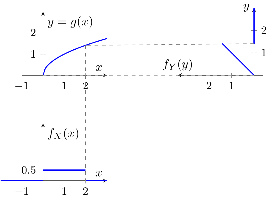
For general non-bijective g, the PDF of Y is: f_Y(y) = \sum_{\nu} \frac{f_X(x_\nu)}{|g'(x_\nu)|} where x_\nu are all solutions of g(x) = y.
Which of the following statements are correct?
- Each solution x_\nu of g(x) = y contributes an additive term f_X(x_\nu)/|g'(x_\nu)| to f_Y(y)
- For Y = X^2 with X symmetric around zero, both x_1 = +\sqrt{y} and x_2 = -\sqrt{y} contribute to f_Y(y) for y > 0
- For Y = \cos(X) with X uniform on [0, 2\pi), the resulting PDF f_Y(y) = \frac{1}{\pi\sqrt{1-y^2}} for |y| < 1 is called the arcsine distribution
- When g is non-bijective, f_Y(y) can only be computed numerically, never in closed form
- The non-bijective formula reduces to the monotone formula when g is strictly monotone, since then there is only one solution x_1 for each y
- ✓ Correct. The total probability density at y is the sum of contributions from all input values that map to y, each weighted by its local stretching factor.
- ✓ Correct. Since g(x) = x^2 maps both +\sqrt{y} and -\sqrt{y} to y, both branches contribute. If X is supported on both sides of zero, both terms appear in the sum.
- ✓ Correct. The cosine mapping has two solutions per y value in (-1,1), and the transformation formula with uniform input yields the arcsine (or bathtub-shaped) distribution.
- ✗ Incorrect. As demonstrated by the quadratic and sinusoidal examples, closed-form expressions for f_Y(y) can often be derived by enumerating all solutions x_\nu and applying the sum formula.
- ✓ Correct. When g is bijective, the sum has only one term, recovering f_Y(y) = f_X(x_1)/|g'(x_1)|.
Correct: For non-bijective mappings, the output PDF is the sum of local monotone contributions — one for each “branch” of the inverse. This generalizes the bijective formula naturally, and many practically relevant cases (quadratic, sinusoidal) admit closed-form results.
Review: Review how the non-bijective formula generalizes the monotone case. Think about which inverse branches contribute for a given output value y.
Q025 Distribution Mapping and Probability Integral Transform
Converting between distributions using the CDF-based mapping
The distribution mapping theorem states: if g(x) = F_Y^{-1}(F_X(x)), then Y = g(X) has CDF F_Y.
Which of the following statements are correct?
- If X has CDF F_X and we set U = F_X(X), then U is uniformly distributed on (0, 1)
- If U is uniform on (0, 1), then X = F_X^{-1}(U) has CDF F_X
- The distribution mapping can transform any continuous RV X into any other continuous RV Y with a strictly increasing CDF
- The probability integral transform works for discrete RVs without modification
- The mapping g(x) = F_Y^{-1}(F_X(x)) requires knowledge of the PDF f_X(x), not just the CDF
- ✓ Correct. This is the probability integral transform (or universality of the uniform). Applying the CDF to its own RV always produces a uniform RV, regardless of the original distribution.
- ✓ Correct. This is the inverse transform method, widely used for generating random samples from any distribution by applying the inverse CDF to uniform random numbers.
- ✓ Correct. The mapping g(x) = F_Y^{-1}(F_X(x)) is well-defined whenever both CDFs are strictly increasing, allowing arbitrary distribution-to-distribution conversion.
- ✗ Incorrect. For discrete RVs, the CDF F_X has jumps, so U = F_X(X) takes only finitely many values and is not uniformly distributed. The probability integral transform in its simple form requires a continuous CDF.
- ✗ Incorrect. The mapping is defined entirely in terms of CDFs (F_X and F_Y^{-1}). No PDF is needed — CDFs suffice.
Correct: The distribution mapping theorem provides a universal method for converting between distributions via the CDF. The probability integral transform (U = F_X(X) is uniform) is the key special case, and its inverse (X = F_X^{-1}(U)) is the basis for random number generation.
Review: Review the two special cases: (1) uniform output via g(x) = F_X(x), and (2) generating from a target CDF via g(u) = F_X^{-1}(u). Consider what happens when the CDF has jumps (discrete case).
Q026 Sum of Independent Random Variables
Understanding the convolution property for PDFs of sums
Let Z = X + Y where X and Y are random variables. Which of the following statements are correct?
- If X and Y are independent, then f_Z(z) = (f_X * f_Y)(z) = \int_{-\infty}^{\infty} f_X(z - w) f_Y(w) \, dw
- The convolution result f_Z = f_X * f_Y holds for any two RVs, regardless of independence
- The result is derived by introducing the auxiliary variable W = Y, applying the Jacobian (which equals 1), and then marginalizing over W
- The moment generating function of Z = X + Y (independent) satisfies \Phi_Z(s) = \Phi_X(s) \cdot \Phi_Y(s)
- If X \sim \mathcal{N}(m_1, \sigma_1^2) and Y \sim \mathcal{N}(m_2, \sigma_2^2) are independent, then Z \sim \mathcal{N}(m_1 m_2, \sigma_1^2 \sigma_2^2)
- ✓ Correct. This is the fundamental convolution result: the PDF of the sum of independent RVs is the convolution of their individual PDFs.
- ✗ Incorrect. The convolution formula requires independence. Without it, the joint density does not factorize, and f_Z(z) = \int f_{XY}(z-w, w) \, dw cannot be simplified to a convolution of marginals.
- ✓ Correct. The transformation (X, Y) \to (Z, W) = (X+Y, Y) has Jacobian determinant 1. The joint density of (Z, W) is f_{XY}(z-w, w), and marginalizing over w yields f_Z(z).
- ✓ Correct. \Phi_Z(s) = \mathbb{E}[e^{s(X+Y)}] = \mathbb{E}[e^{sX}] \cdot \mathbb{E}[e^{sY}] by independence. This multiplication in the transform domain corresponds to convolution in the density domain.
- ✗ Incorrect. For independent Gaussians, Z = X + Y \sim \mathcal{N}(m_1 + m_2, \sigma_1^2 + \sigma_2^2). The means and variances add, they do not multiply.
Correct: The convolution property is one of the most important results in probability: independent sums yield convoluted PDFs. In the transform domain, convolution becomes multiplication of MGFs (or characteristic functions). For Gaussians, this means means add and variances add.
Review: Remember: PDFs convolve, MGFs multiply. For Gaussians, the sum has mean m_1 + m_2 and variance \sigma_1^2 + \sigma_2^2 — addition, not multiplication.
Q027 Multivariate Transformation and the Jacobian
Understanding the change-of-variables theorem for random vectors
For a bijective transformation \mathbf{Y} = \mathbf{g}(\mathbf{X}) of a random vector, the joint PDF transforms as:
f_{\mathbf{Y}}(\mathbf{y}) = \frac{f_{\mathbf{X}}(\mathbf{x})}{|J(\mathbf{x})|}, \quad J(\mathbf{x}) = \det\!\left(\frac{\partial \mathbf{g}}{\partial \mathbf{x}}\right)
Which of the following statements are correct?
- The Jacobian determinant |J(\mathbf{x})| measures how much the transformation locally stretches or compresses volume
- The Jacobian transformation requires that the input and output vectors have the same dimension
- If the Jacobian determinant |J| = 1, the density is unchanged: f_{\mathbf{Y}}(\mathbf{y}) = f_{\mathbf{X}}(\mathbf{x})
- The Jacobian formula can be applied even when the mapping is not bijective, as long as it is differentiable
- For the transformation Z = \max(X, Y) with independent RVs, we can directly apply the Jacobian formula
- ✓ Correct. A small volume element d\mathbf{x} is mapped to d\mathbf{y} = |J| \, d\mathbf{x}. Since probability mass is preserved, the density is divided by this volume scaling factor.
- ✓ Correct. A bijective mapping with a well-defined square Jacobian matrix and nonzero determinant requires \dim(\mathbf{X}) = \dim(\mathbf{Y}). Dimension reduction requires marginalization instead.
- ✓ Correct. When |J| = 1, the transformation preserves volume, so densities are preserved (evaluated at the corresponding points). This occurs, e.g., for the sum transformation (Z,W) = (X+Y, Y).
- ✗ Incorrect. The Jacobian formula requires bijectivity. For non-bijective mappings (dimension reduction or multiple pre-images), different techniques are needed — either summing over branches (like the non-bijective 1D formula) or marginalizing auxiliary variables.
- ✗ Incorrect. Z = \max(X, Y) reduces two variables to one (dimension reduction), and the max function is not bijective. Instead, the CDF approach F_Z(z) = \mathbb{P}(X \leq z, Y \leq z) = F_X(z) F_Y(z) is used.
Correct: The Jacobian formula generalizes the 1D transformation rule to multiple dimensions. It requires equal input/output dimensions and bijectivity. The determinant quantifies the local volume change, preserving total probability under the transformation.
Review: Recall that the Jacobian formula requires a bijective (one-to-one and onto) mapping. For operations like max, which reduce dimensionality, the CDF approach or marginalization is needed instead.
§ 2.4 Expectations
Q028 The Expectation Operator and Its Linearity
Understanding the definition and properties of the expectation
Which of the following statements about the expectation operator \mathbb{E}[g(X)] = \int g(x) f_X(x) \, dx are correct?
- \mathbb{E}[a_1 g_1(X) + a_2 g_2(Y)] = a_1 \mathbb{E}[g_1(X)] + a_2 \mathbb{E}[g_2(Y)] holds for any RVs X, Y and constants a_1, a_2
- The linearity of \mathbb{E}[\cdot] allows interchanging the order of expectation with other linear operators like convolution and Fourier transforms
- \mathbb{E}[g(X)] = g(\mathbb{E}[X]) for any function g
- For a constant c, \mathbb{E}[c] = c
- The expectation \mathbb{E}[X] always exists (is finite) for any RV X
- ✓ Correct. The expectation operator is linear, and this property holds regardless of whether X and Y are independent or not. It follows from the linearity of integration.
- ✓ Correct. Since \mathbb{E}[\cdot] is a linear operator, it commutes with other linear operations (assuming convergence), which is crucial for analyzing LTI systems with stochastic inputs.
- ✗ Incorrect. In general, \mathbb{E}[g(X)] \neq g(\mathbb{E}[X]). Equality holds only when g is affine (linear). For example, \mathbb{E}[X^2] \neq (\mathbb{E}[X])^2 unless \text{Var}(X) = 0. This error is sometimes called the “fallacy of the average.”
- ✓ Correct. A constant is not random, so \mathbb{E}[c] = c \int f_X(x) \, dx = c \cdot 1 = c.
- ✗ Incorrect. Some distributions, like the Cauchy distribution, have no finite mean because \int |x| f_X(x) \, dx = \infty. The expectation exists only when the integral converges absolutely.
Correct: Linearity is the most important property of the expectation operator. It holds unconditionally (no independence required) and enables powerful manipulations with linear systems. However, expectation does not commute with nonlinear functions, and some distributions lack finite moments.
Review: Be careful with \mathbb{E}[g(X)] \neq g(\mathbb{E}[X]) for nonlinear g. Also recall that not all distributions have finite moments (Cauchy has no mean, no variance).
Q029 Mean and Variance
Understanding the first two moments and their fundamental relationship
Which of the following statements about the mean m_X = \mathbb{E}[X] and variance \sigma_X^2 = \mathbb{E}[(X - m_X)^2] are correct?
- The variance can be computed as \sigma_X^2 = \mathbb{E}[X^2] - (\mathbb{E}[X])^2 = m_X^{(2)} - m_X^2
- The mean m_X corresponds to the center of mass of the PDF
- The variance is always non-negative, and \sigma_X^2 = 0 implies X = m_X with probability 1 (a deterministic constant)
- For a symmetric PDF, all moments are zero
- The variance satisfies \sigma_X^2 = m_X^{(2)} - m_X^2, which implies \mathbb{E}[X^2] \geq (\mathbb{E}[X])^2
- ✓ Correct. Expanding (X - m_X)^2 and using linearity of expectation gives \sigma_X^2 = \mathbb{E}[X^2] - 2m_X\mathbb{E}[X] + m_X^2 = m_X^{(2)} - m_X^2.
- ✓ Correct. Just as the center of mass of a mass distribution is the weighted average of positions, m_X = \int x \, f_X(x) \, dx is the weighted average of values with the PDF as the weight function.
- ✓ Correct. \sigma_X^2 = \mathbb{E}[(X-m_X)^2] \geq 0 since we are averaging a non-negative quantity. It equals zero only when X deviates from m_X with zero probability.
- ✗ Incorrect. For a symmetric PDF (f_X(x) = f_X(-x)), only the odd-order moments (n = 1, 3, 5, \ldots) are zero. Even-order moments (like m_X^{(2)}) are generally nonzero; for example, the variance of a symmetric distribution is typically positive.
- ✓ Correct. Since \sigma_X^2 \geq 0, we have m_X^{(2)} \geq m_X^2, i.e., the second moment is always at least as large as the square of the first moment. This is a consequence of Jensen’s inequality.
Correct: The mean and variance are the two most fundamental descriptors of a distribution: the center and the spread. The shortcut formula \sigma_X^2 = \mathbb{E}[X^2] - m_X^2 is practically very useful. For symmetric distributions, only odd-order moments vanish, not all moments.
Review: A symmetric PDF has f_X(x-m_X) = f_X(-(x-m_X)), which makes only odd-order central moments vanish. Even-order moments like variance measure spread and are generally nonzero.
Q030 Skewness and Kurtosis
Understanding higher-order moments and their interpretation
Skewness is defined as \mu_X^{(3)} = \mathbb{E}[(X - m_X)^3] and kurtosis as \kappa(X) = \mu_X^{(4)} - 3\sigma_X^4. Which of the following statements are correct?
- A positive kurtosis (\kappa > 0) indicates a super-Gaussian distribution with heavier tails than a Gaussian of the same variance
- The kurtosis of a Gaussian distribution is zero
- The uniform distribution is super-Gaussian because it has heavier tails than the Gaussian
- Skewness is zero for any PDF that is symmetric about its mean
- The Laplace distribution has kurtosis \kappa = 3\sigma_X^4 > 0, confirming it is super-Gaussian
- ✓ Correct. Super-Gaussian distributions (e.g., Laplace) have heavier tails, meaning large deviations from the mean are more likely than for a Gaussian. This is captured by \kappa > 0.
- ✓ Correct. By definition, kurtosis compares the fourth central moment to 3\sigma_X^4 (the fourth central moment of a Gaussian). For a Gaussian, \mu_X^{(4)} = 3\sigma_X^4, so \kappa = 0.
- ✗ Incorrect. The uniform distribution has \kappa = -6\sigma_X^4/5 < 0, making it sub-Gaussian (platykurtic). It has lighter tails than the Gaussian — in fact, it has no tails at all, being bounded.
- ✓ Correct. For a symmetric PDF, f_X(x - m_X) = f_X(-(x - m_X)), so all odd central moments (including \mu_X^{(3)}) vanish.
- ✓ Correct. The Laplace distribution has \mu_X^{(4)} = 6\sigma_X^4, so \kappa = 6\sigma_X^4 - 3\sigma_X^4 = 3\sigma_X^4 > 0, confirming its heavy-tailed (super-Gaussian) nature.
Correct: Kurtosis measures tail heaviness relative to the Gaussian: \kappa > 0 (super-Gaussian, heavy tails), \kappa = 0 (Gaussian), \kappa < 0 (sub-Gaussian, light tails). Skewness measures asymmetry and vanishes for symmetric distributions. The uniform distribution is sub-Gaussian despite being a simple “baseline” distribution.
Review: Review the kurtosis values: Uniform (\kappa < 0, sub-Gaussian), Gaussian (\kappa = 0), Laplace (\kappa > 0, super-Gaussian). “Heavy tails” means more probability mass far from the mean, not wider support.
Q031 Power Means: Arithmetic, Geometric, and Harmonic
Understanding the ordering and applications of different types of means
The power mean of a positive RV X is defined as m_{X,p} = (\mathbb{E}[X^p])^{1/p}. Which of the following statements are correct?
- The ordering m_{X,\text{arithmetic}} \geq m_{X,\text{geometric}} \geq m_{X,\text{harmonic}} always holds for positive RVs
- The geometric mean is obtained as p \to 0 and equals \exp(\mathbb{E}[\ln X])
- The harmonic mean (p = -1) is the most appropriate mean for averaging speeds when distances are equal
- For a constant RV (X = c with probability 1), all power means are equal to c
- The arithmetic mean is always the best choice for summarizing any dataset, regardless of the underlying structure
- ✓ Correct. The power mean m_{X,p} is monotonically non-decreasing in p. Since arithmetic (p=1), geometric (p \to 0), and harmonic (p=-1) correspond to decreasing p, the stated ordering follows.
- ✓ Correct. Taking the limit p \to 0 of (\mathbb{E}[X^p])^{1/p} leads to \exp(\mathbb{E}[\ln X]), which is the geometric mean.
- ✓ Correct. When averaging quotients (like speed = distance/time) over equal distances, the harmonic mean correctly weights by the time spent at each speed, yielding the true average speed.
- ✓ Correct. When there is no variability, m_{X,p} = (\mathbb{E}[c^p])^{1/p} = c for all p. The inequality between means becomes equality only when the RV is deterministic.
- ✗ Incorrect. The arithmetic mean is appropriate for additive quantities, but for multiplicatively linked quantities (e.g., growth rates, interest rates), the geometric mean is correct, and for averaging rates (e.g., speeds over equal distances), the harmonic mean is appropriate.
Correct: Different means are appropriate for different structures: arithmetic for additive, geometric for multiplicative, harmonic for rate-based quantities. The power mean framework unifies them and establishes their universal ordering for positive random variables.
Review: Consider the cyclist example from the lecture: why does the arithmetic mean of speeds overestimate the actual average speed? The time spent at each speed varies, which is what the harmonic mean correctly accounts for.
Q032 Moment Generating Function
Understanding the MGF, the moment theorem, and its relationship to transforms
The moment generating function (MGF) is defined as \Phi_X(s) = \mathbb{E}[e^{sX}]. Which of the following statements are correct?
- The n-th moment of X is obtained by m_X^{(n)} = \Phi_X^{(n)}(0), i.e., the n-th derivative of \Phi_X(s) evaluated at s = 0
- The characteristic function \Phi_X(j\omega) = \mathbb{E}[e^{j\omega X}] is the Fourier transform of the PDF f_X(-x)
- For independent RVs Z = X + Y, the MGF factorizes: \Phi_Z(s) = \Phi_X(s) \cdot \Phi_Y(s)
- The MGF always exists (is finite) for any distribution
- The MGF of a Gaussian \mathcal{N}(m, \sigma^2) is \Phi_X(s) = e^{sm + s^2\sigma^2/2}
- ✓ Correct. This is the moment theorem. Expanding e^{sX} as a Taylor series \sum \frac{(sX)^n}{n!} and taking derivatives recovers each moment.
- ✓ Correct. Comparing \Phi_X(j\omega) = \int f_X(x) e^{j\omega x} dx with the standard Fourier transform definition shows it equals \mathcal{F}\{f_X(-x)\}.
- ✓ Correct. By independence, \Phi_Z(s) = \mathbb{E}[e^{s(X+Y)}] = \mathbb{E}[e^{sX}] \cdot \mathbb{E}[e^{sY}]. This multiplication in the transform domain corresponds to convolution of PDFs.
- ✗ Incorrect. The MGF \Phi_X(s) = \int f_X(x) e^{sx} dx may diverge for heavy-tailed distributions. For example, the Cauchy distribution has no finite MGF. The characteristic function (s = j\omega), however, always exists.
- ✓ Correct. This can be verified by completing the square in the integral \int \frac{1}{\sqrt{2\pi}\sigma} e^{-(x-m)^2/(2\sigma^2)} e^{sx} dx.
Correct: The MGF encodes all moments in a single function and transforms convolution of PDFs into multiplication. It is related to the Laplace/Fourier transform of the PDF. Unlike the MGF, the characteristic function (s = j\omega) always exists.
Review: Recall that the MGF involves e^{sx} which can grow without bound for heavy-tailed distributions. The characteristic function uses e^{j\omega x} (bounded oscillation), so it always exists.
Q033 Cumulants and Gaussian Random Variables
Understanding the cumulant generating function and why Gaussians are special
The cumulant generating function (CGF) is \Psi_X(s) = \ln \Phi_X(s), and cumulants are \lambda_X^{(n)} = \Psi_X^{(n)}(0).
Which of the following statements are correct?
- For a Gaussian RV, \lambda_X^{(1)} = m_X, \lambda_X^{(2)} = \sigma_X^2, and all higher cumulants (n > 2) are zero
- For independent RVs Z = X + Y, cumulants add: \lambda_Z^{(n)} = \lambda_X^{(n)} + \lambda_Y^{(n)}
- The fourth cumulant \lambda_X^{(4)} equals the kurtosis \kappa(X) for zero-mean RVs
- Moments and cumulants are always identical: \lambda_X^{(n)} = m_X^{(n)} for all n
- The fact that all Gaussian cumulants beyond order 2 vanish means a Gaussian distribution is fully characterized by its mean and variance
- ✓ Correct. The Gaussian CGF is \Psi_X(s) = sm_X + s^2\sigma_X^2/2, which is a polynomial of degree 2 in s. All derivatives of order n > 2 vanish.
- ✓ Correct. Since \Phi_Z = \Phi_X \Phi_Y for independent RVs, \Psi_Z = \ln \Phi_Z = \ln \Phi_X + \ln \Phi_Y = \Psi_X + \Psi_Y. Hence all cumulants add.
- ✓ Correct. For zero-mean RVs, \lambda_X^{(4)} = \mu_X^{(4)} - 3\sigma_X^4 = \kappa(X). The fourth cumulant thus measures the deviation of the tail behavior from that of a Gaussian.
- ✗ Incorrect. Moments and cumulants agree only for n = 1 (\lambda_X^{(1)} = m_X^{(1)}). For n \geq 2, cumulants involve combinations of lower moments. For example, \lambda_X^{(2)} = m_X^{(2)} - (m_X^{(1)})^2 = \sigma_X^2.
- ✓ Correct. Since \Psi_X(s) = sm_X + s^2\sigma_X^2/2 depends only on m_X and \sigma_X^2, and the CGF uniquely determines the distribution, knowing the first two cumulants is sufficient for a Gaussian.
Correct: Cumulants provide a compact characterization of distributions. The Gaussian is uniquely simple: only two nonzero cumulants. The additivity of cumulants under independent sums is a key advantage over moments. The fourth cumulant directly measures non-Gaussianity (kurtosis).
Review: Cumulants are related to moments but are not the same. The key relationship is \Psi_X = \ln \Phi_X, so cumulants involve logarithmic combinations of moments. Compare the first few explicitly.
Q034 Correlation and Covariance
Understanding the fundamental second-order joint moments
For two RVs X and Y with means m_X, m_Y, the correlation is R_{XY} = \mathbb{E}[XY] and the covariance is C_{XY} = \mathbb{E}[(X - m_X)(Y - m_Y)].
Which of the following statements are correct?
- C_{XY} = \mathbb{E}[XY] - m_X \cdot m_Y = R_{XY} - m_X m_Y
- Two RVs are uncorrelated if and only if C_{XY} = 0, which is equivalent to \mathbb{E}[XY] = \mathbb{E}[X] \cdot \mathbb{E}[Y]
- A positive covariance C_{XY} > 0 means that Y increases whenever X increases, with certainty
- If X and Y are independent, then R_{XY} = 0
- The covariance of a RV with itself equals its variance: C_{XX} = \sigma_X^2
- ✓ Correct. Expanding the product (X - m_X)(Y - m_Y) and applying linearity of expectation yields C_{XY} = \mathbb{E}[XY] - m_X m_Y.
- ✓ Correct. Uncorrelatedness means zero covariance, and from C_{XY} = \mathbb{E}[XY] - m_Xm_Y = 0, the factorization of the mixed moment follows.
- ✗ Incorrect. Positive covariance means that on average, X and Y tend to deviate from their means in the same direction. It does not guarantee a deterministic relationship for every realization.
- ✗ Incorrect. Independence implies \mathbb{E}[XY] = \mathbb{E}[X]\mathbb{E}[Y], so R_{XY} = m_X m_Y, which is zero only if at least one mean is zero. Independence implies zero covariance, not zero correlation.
- ✓ Correct. Setting Y = X in the definition gives C_{XX} = \mathbb{E}[(X - m_X)^2] = \sigma_X^2.
Correct: Correlation and covariance are related by C_{XY} = R_{XY} - m_Xm_Y. Uncorrelatedness means zero covariance (expectation factorizes), which is a weaker condition than independence. Be careful to distinguish between correlation (\mathbb{E}[XY]) and covariance (\mathbb{E}[(X-m_X)(Y-m_Y)]).
Review: Independence implies \mathbb{E}[XY] = \mathbb{E}[X]\mathbb{E}[Y] (zero covariance), but \mathbb{E}[XY] itself is zero only when at least one mean is zero. Review the difference between correlation and covariance.
Q036 Correlation Coefficient and Cauchy–Schwarz Inequality
Understanding the normalized measure of linear dependence
The correlation coefficient is defined as c_{XY} = C_{XY} / (\sigma_X \sigma_Y) with |c_{XY}| \leq 1 (Cauchy–Schwarz inequality).
Which of the following statements are correct?
- |c_{XY}| = 1 if and only if Y = aX + b for some constants a \neq 0 and b, i.e., a perfect linear relationship exists
- c_{XY} = 0 implies that X and Y are independent
- The correlation coefficient measures the strength of the linear relationship between X and Y
- A strong correlation proves a causal relationship between X and Y
- The Cauchy–Schwarz inequality |\mathbb{E}[UV^*]|^2 \leq \mathbb{E}[|U|^2] \cdot \mathbb{E}[|V|^2] holds for both real and complex RVs
- ✓ Correct. Equality in Cauchy–Schwarz occurs when one centered RV is a scalar multiple of the other: Y - m_Y = \lambda(X - m_X), which gives a perfect linear relationship.
- ✗ Incorrect. c_{XY} = 0 means uncorrelatedness (zero linear dependence), but nonlinear dependencies can still exist. For example, X and Y = X^2 with X symmetric have c_{XY} = 0 but are clearly dependent.
- ✓ Correct. The correlation coefficient quantifies how well Y can be predicted by a linear function of X. It does not capture nonlinear relationships.
- ✗ Incorrect. Correlation reflects statistical association, not causation. A strong correlation may arise from confounding variables, coincidence, or indirect causal chains. “Correlation does not imply causation.”
- ✓ Correct. The Cauchy–Schwarz inequality for expectations is a general result that applies to both real and complex random variables with finite second moments.
Correct: The correlation coefficient is a standardized measure of linear dependence, bounded by [-1, 1] via Cauchy–Schwarz. It detects linear relationships perfectly but is blind to nonlinear dependencies. Correlation does not establish causation.
Review: Recall that uncorrelatedness (c_{XY} = 0) is weaker than independence. Think of the Y = X^2 counterexample. Also remember: “correlation suggests, but does not prove, a relationship.”
Q037 Conditional Expectation
Understanding conditional expectations and their properties
Which of the following statements about the conditional expectation \mathbb{E}[X | Y = y] are correct?
- The conditional mean m_{X|Y=y} = \mathbb{E}[X | Y = y] = \int x \, f_{X|Y}(x|y) \, dx is in general a function of y
- If X and Y are independent, then \mathbb{E}[X | Y = y] = \mathbb{E}[X] for all y
- \mathbb{E}[X | X] = X almost surely
- The conditional expectation \mathbb{E}[X | Y] is a constant (a number), not a random variable
- For a nonlinear sensor Y = g(X) + N with independent noise N, the conditional expectation \mathbb{E}[X | Y = y] provides the optimal estimator in the mean-square sense
- ✓ Correct. For each fixed y, the conditional density f_{X|Y}(x|y) may differ, producing a different conditional mean. The function \Theta(y) = \mathbb{E}[X | Y = y] is called the regression function.
- ✓ Correct. Independence means f_{X|Y}(x|y) = f_X(x), so conditioning on Y provides no information about X, and the conditional mean reduces to the unconditional mean.
- ✓ Correct. Conditioning a RV on itself reveals its value with certainty, so no averaging is needed: \mathbb{E}[X | X = x] = x for all x in the support.
- ✗ Incorrect. While \mathbb{E}[X | Y = y] is a number for fixed y, the conditional expectation \mathbb{E}[X | Y] = \Theta(Y) is a function of the random variable Y, and hence is itself a random variable.
- ✓ Correct. The conditional expectation minimizes \mathbb{E}[(X - \hat{X})^2] over all measurable functions of Y, making it the MMSE estimator.
Correct: Conditional expectation is a versatile concept: it is a function of y when y is fixed, and a random variable when Y is random. It reduces to the unconditional mean under independence and to the value itself when conditioned on X = x. It serves as the optimal estimator in the MSE sense.
Review: Distinguish between \mathbb{E}[X | Y = y] (a number for each y) and \mathbb{E}[X | Y] (a random variable, since Y is random). The latter is a function of the random Y.
Q038 Moments of Complex Random Variables
Understanding absolute moments, pseudo-variance, and power for complex RVs
For a complex RV Z = X + jY (or Z = R \cdot e^{j\Phi}), which of the following statements are correct?
- The average power of Z is given by \mathbb{E}[|Z|^2] = \mathbb{E}[ZZ^*] = \mathbb{E}[X^2] + \mathbb{E}[Y^2]
- If the phase \Phi is uniformly distributed on [0, 2\pi) and independent of R, then all (non-absolute) moments m_Z^{(n)} = \mathbb{E}[Z^n] are zero for n \geq 1
- The quantity \mathbb{E}[Z^2] is the variance of Z
- For M-ary PSK symbols w_k = e^{j2\pi k/M} transmitted with equal probability, the average symbol power is \mathbb{E}[WW^*] = 1
- The covariance C_{ZZ} = \mathbb{E}[(Z - \mathbb{E}[Z])(Z^* - \mathbb{E}[Z^*])] is always a complex number
- ✓ Correct. ZZ^* = (X+jY)(X-jY) = X^2 + Y^2, so \mathbb{E}[|Z|^2] = \mathbb{E}[X^2] + \mathbb{E}[Y^2]. The cross-term \mathbb{E}[XY] does not appear.
- ✓ Correct. The integral \frac{1}{2\pi}\int_0^{2\pi} e^{jn\phi} d\phi = 0 for n \neq 0, making the phase factor vanish and hence m_Z^{(n)} = 0.
- ✗ Incorrect. \mathbb{E}[Z^2] is called the pseudo-variance and involves the cross-term \mathbb{E}[X^2] - \mathbb{E}[Y^2] + 2j\mathbb{E}[XY]. The proper variance of a complex RV is \sigma_Z^2 = \mathbb{E}[|Z - m_Z|^2] = \mathbb{E}[(Z - m_Z)(Z^* - m_Z^*)].
- ✓ Correct. WW^* = |w_k|^2 = |e^{j2\pi k/M}|^2 = 1 for all k, so the average power is \frac{1}{M}\sum_{k=0}^{M-1} 1 = 1.
- ✗ Incorrect. C_{ZZ} = \mathbb{E}[|Z - m_Z|^2] = C_{XX} + C_{YY}, which is always real and non-negative (sum of two variances), just like the variance for real RVs.
Correct: For complex RVs, the absolute moment \mathbb{E}[|Z|^2] (using conjugation) gives the correct power. The ordinary moment \mathbb{E}[Z^2] (pseudo-variance) is generally complex and does not represent power. The covariance C_{ZZ} is always real since it equals C_{XX} + C_{YY}.
Review: Distinguish between \mathbb{E}[Z^2] (pseudo-variance, generally complex) and \mathbb{E}[|Z|^2] = \mathbb{E}[ZZ^*] (power, always real). The proper variance of a complex RV uses the conjugate: \mathbb{E}[(Z-m_Z)(Z^*-m_Z^*)].
§ 2.5 Special Distributions
Q039 Binomial Distribution
Understanding the binomial distribution Bin(N,p), its parameters, and its connection to Bernoulli trials
Which of the following statements about the binomial distribution \text{Bin}(N,p) are correct?
The binomial distribution describes the number of successes in N independent Bernoulli trials, each with success probability p. Its probability mass function is: \mathbb{P}(X = k) = \binom{N}{k} p^k (1-p)^{N-k}, \quad k = 0, 1, \ldots, N
- The mean of a binomial random variable X \sim \text{Bin}(N,p) is m_X = Np
- The variance of a binomial random variable is \sigma_X^2 = Np(1-p)
- A binomial RV X can be written as X = \sum_{i=1}^{N} X_i where X_i are independent Bernoulli trials with success probability p
- The variance of a binomial random variable is \sigma_X^2 = Np^2
- The binomial distribution requires continuous-valued outcomes
- ✓ Correct. Since X is the sum of N independent Bernoulli RVs each with mean p, linearity of expectation gives m_X = Np.
- ✓ Correct. Each Bernoulli trial has variance p(1-p), and since the trials are independent, the variances add up to Np(1-p).
- ✓ Correct. This is precisely the definition: a binomial RV is the sum of N independent, identically distributed Bernoulli random variables.
- ✗ Incorrect. The variance is Np(1-p), not Np^2. This would overestimate the variance for all p < 1.
- ✗ Incorrect. The binomial distribution is a discrete distribution — X takes integer values from 0 to N.
Correct: The binomial distribution is a fundamental discrete distribution arising from repeated independent Bernoulli trials. Its mean Np and variance Np(1-p) follow directly from the additivity of expectations and variances of independent random variables.
Review: Review how the binomial distribution is constructed from independent Bernoulli trials. Remember that the variance of a Bernoulli RV with parameter p is p(1-p), and that the binomial distribution is always discrete.
Q040 De Moivre–Laplace Theorem
Understanding the convergence of the binomial distribution to the Gaussian as the number of trials grows
Which of the following statements about the de Moivre–Laplace theorem are correct?
The theorem concerns the behavior of a properly normalized binomial random variable X \sim \text{Bin}(N,p) as N \to \infty, under the condition that Np(1-p) \gg 1.
- The normalized binomial \frac{X - Np}{\sqrt{Np(1-p)}} converges in distribution to a standard normal \mathcal{N}(0,1) as N \to \infty
- The Galton board (bean machine) provides a physical demonstration of this theorem for p = 0.5
- The convergence of the de Moivre–Laplace theorem is pointwise convergence of the PMF to the Gaussian PDF
- The de Moivre–Laplace theorem only applies when p = 0.5
- As N increases, the binomial PMF itself becomes exactly a Gaussian PDF
- ✓ Correct. This is the statement of the de Moivre–Laplace theorem: the CDF of the normalized binomial converges pointwise to the standard normal CDF.
- ✓ Correct. In a Galton board, a ball falls through rows of pins with equal probability of going left or right (p = 0.5), and the resulting distribution of positions approximates a Gaussian for many rows.
- ✗ Incorrect. Convergence in distribution means convergence of CDFs, not pointwise convergence of PMF to PDF. A discrete PMF cannot converge to a continuous PDF.
- ✗ Incorrect. The theorem holds for any fixed p \in (0,1) as long as Np(1-p) \gg 1, not just for the symmetric case.
- ✗ Incorrect. The binomial remains a discrete distribution for any finite N. The theorem states convergence in distribution (CDF convergence) of the normalized variable, not that the PMF transforms into a PDF.
Correct: The de Moivre–Laplace theorem is a special case of the Central Limit Theorem applied to Bernoulli trials. The key insight is that convergence is in distribution (CDF convergence), and it applies for any success probability p, not just the symmetric case.
Review: Remember the distinction between convergence in distribution (CDF convergence) and pointwise convergence of density/mass functions. Also note that the theorem applies to any fixed p \in (0,1), not only the symmetric case.
Q041 Geometric Distribution
Understanding the geometric distribution, its support, and its mean
Which of the following statements about the geometric distribution are correct?
In the lecture, the geometric distribution is defined as the number of failures X before the first success in a sequence of independent Bernoulli trials with success probability p: \mathbb{P}(X = k) = p(1-p)^k, \quad k = 0, 1, 2, \ldots
- Each trial outcome is independent of all previous trial outcomes
- The mean number of failures before the first success is m_X = \frac{1-p}{p}
- The geometric distribution has a finite support (i.e., a maximum possible value)
- The mean number of failures before the first success is m_X = \frac{p}{1-p}
- The geometric distribution requires specifying a fixed number of trials N in advance, similar to the binomial distribution
- ✓ Correct. The geometric distribution arises from a sequence of independent Bernoulli trials — each trial’s outcome does not depend on the results of prior trials.
- ✓ Correct. For the geometric distribution counting failures (starting from k = 0), the mean is (1-p)/p.
- ✗ Incorrect. The geometric distribution has infinite support — k can be any non-negative integer. In principle, one might have to wait arbitrarily long for the first success.
- ✗ Incorrect. The correct mean is (1-p)/p, not p/(1-p). For small p, one expects many failures on average, so the mean should grow as p \to 0.
- ✗ Incorrect. Unlike the binomial distribution, the geometric distribution does not fix the number of trials. The experiment continues until the first success, with no predetermined limit.
Correct: The geometric distribution models waiting for the first success in a sequence of independent Bernoulli trials. Its infinite support reflects the fact that success is never guaranteed by any specific trial. The mean (1-p)/p makes intuitive sense: rare events (p small) require many failures on average.
Review: Review the definition of the geometric distribution and how it differs from the binomial. Pay attention to whether the support is bounded, and check the formula for the mean by considering limiting cases (p \to 0 and p \to 1).
Q042 Poisson Distribution
Understanding the Poisson distribution, its properties, and its connection to the binomial distribution
Which of the following statements about the Poisson distribution are correct?
The Poisson distribution with parameter a > 0 has the probability mass function: \mathbb{P}(X = k) = \frac{a^k}{k!} e^{-a}, \quad k = 0, 1, 2, \ldots
- The mean and variance of the Poisson distribution are both equal to a
- The Poisson distribution arises as a limit of the binomial \text{Bin}(N,p) when N \to \infty and p \to 0 such that Np = a remains constant
- The Poisson distribution is widely used for counting events such as photon arrivals or radioactive decays
- The Poisson distribution has mean a but variance a^2
- The Poisson distribution is a continuous distribution
- ✓ Correct. A defining characteristic of the Poisson distribution is that its mean and variance are identical: m_X = \sigma_X^2 = a.
- ✓ Correct. This is the Poisson limit theorem — the Poisson approximation to the binomial for rare events with many trials.
- ✓ Correct. The Poisson distribution naturally models the count of independent rare events occurring in a fixed interval (e.g., photon counting, particle detection).
- ✗ Incorrect. The variance of the Poisson distribution is a, not a^2. Mean and variance being equal is a hallmark of the Poisson distribution.
- ✗ Incorrect. The Poisson distribution is discrete — it assigns probabilities to non-negative integers k = 0, 1, 2, \ldots
Correct: The Poisson distribution is one of the most important discrete distributions. It arises naturally as the limit of binomial trials when events are rare (p \to 0) but opportunities are many (N \to \infty). Its equal mean and variance are a distinctive signature often used to identify Poisson-distributed data.
Review: Review the Poisson limit theorem and the properties of the Poisson distribution. Remember that it is a discrete distribution and that its mean equals its variance — this is a unique and important property.
Q043 Special Properties of the Gaussian Distribution
Understanding the unique properties of the Gaussian (normal) distribution
Which of the following statements about the Gaussian (normal) distribution are correct?
Consider the properties that make the Gaussian distribution uniquely important in probability and statistics.
- Approximately 68% of the probability mass lies within one standard deviation of the mean, and approximately 95% within two standard deviations
- The sum of independent Gaussian random variables is again Gaussian
- The Central Limit Theorem explains why the Gaussian distribution appears so frequently in practice
- For jointly Gaussian random variables, uncorrelatedness implies statistical independence
- Any two uncorrelated random variables that are each marginally Gaussian must be statistically independent
- ✓ Correct. These are the well-known 68–95–99.7 percentages for the Gaussian distribution at \pm 1\sigma, \pm 2\sigma, and \pm 3\sigma.
- ✓ Correct. The Gaussian family is closed under convolution: if X \sim \mathcal{N}(m_1, \sigma_1^2) and Y \sim \mathcal{N}(m_2, \sigma_2^2) are independent, then X + Y \sim \mathcal{N}(m_1 + m_2, \sigma_1^2 + \sigma_2^2).
- ✓ Correct. By the CLT, sums of many independent random variables tend toward a Gaussian distribution regardless of the original distributions, which is why it arises so ubiquitously.
- ✓ Correct. This is a special property unique to the Gaussian distribution. In general, uncorrelated does not imply independent — but for jointly Gaussian RVs, it does.
- ✗ Incorrect. The implication “uncorrelated \Rightarrow independent” requires that the variables are jointly Gaussian. Two marginally Gaussian RVs can be uncorrelated yet dependent if their joint distribution is not Gaussian.
Correct: The Gaussian distribution has a unique combination of properties: closure under addition, the 68–95–99.7 rule, and the equivalence of uncorrelatedness and independence for jointly Gaussian vectors. The CLT provides the theoretical justification for its ubiquity.
Review: Pay careful attention to the distinction between marginally Gaussian and jointly Gaussian random variables. The special property that uncorrelated implies independent only holds when the joint distribution is Gaussian, not merely when each marginal is Gaussian.
Q044 Gaussian Mixture Distributions
Understanding Gaussian mixture models, their properties, and applications
Which of the following statements about Gaussian mixture distributions are correct?
A Gaussian mixture distribution has the PDF: f_X(x) = \sum_{i=1}^{K} \alpha_i \, \mathcal{N}(x; \mu_i, \sigma_i^2) where \alpha_i > 0 are the mixture weights and \mathcal{N}(x; \mu_i, \sigma_i^2) denotes a Gaussian PDF with mean \mu_i and variance \sigma_i^2.
- The mixture weights must satisfy \sum_{i=1}^{K} \alpha_i = 1
- Gaussian mixtures can model multimodal distributions (distributions with multiple peaks)
- A Gaussian mixture distribution is itself a Gaussian distribution
- Gaussian mixture distributions are always unimodal (single-peaked)
- The mean of a Gaussian mixture always equals the average of the component means, i.e., m_X = \frac{1}{K}\sum_{i=1}^{K} \mu_i
- ✓ Correct. Since f_X(x) must integrate to 1, and each component \mathcal{N}(x; \mu_i, \sigma_i^2) integrates to 1, the weights must sum to 1.
- ✓ Correct. By choosing components with well-separated means, a Gaussian mixture can produce multiple distinct peaks, making it a flexible model for multimodal data such as impulsive noise.
- ✗ Incorrect. A mixture of Gaussians is generally not Gaussian. The resulting PDF can be multimodal, skewed, or have heavier tails — none of which are properties of a single Gaussian.
- ✗ Incorrect. A key advantage of Gaussian mixtures is precisely their ability to represent multimodal distributions with multiple peaks.
- ✗ Incorrect. The mean of a mixture is the weighted average m_X = \sum_{i=1}^{K} \alpha_i \mu_i. It equals the simple average only when all weights are equal (\alpha_i = 1/K).
Correct: Gaussian mixtures are a powerful and flexible class of distributions formed by combining weighted Gaussian components. They can represent multimodal, skewed, and heavy-tailed distributions, and are widely used to model impulsive noise and heterogeneous data.
Review: Remember that mixing Gaussians does not produce a Gaussian in general. Also, the overall mean depends on the mixture weights, not just the component means. Review how the weights influence the shape and moments of the mixture.
Q045 Cauchy Distribution
Understanding the Cauchy distribution and its unusual moment properties
Which of the following statements about the Cauchy distribution are correct?
The Cauchy distribution has the PDF: f_X(x) = \frac{b}{\pi\big(b^2 + (x - a)^2\big)} where a is the location parameter and b > 0 is the scale parameter. It arises, for example, as the ratio of two independent standard normal random variables.
- The Cauchy distribution has no finite mean or variance — all moments are undefined
- The mean of the Cauchy distribution is m_X = a
- The variance of the Cauchy distribution is \sigma_X^2 = b^2
- The Cauchy distribution has lighter tails than the Gaussian distribution
- The sample mean of i.i.d. Cauchy random variables converges to a by the Law of Large Numbers
- ✓ Correct. The integral \int x \, f_X(x)\,dx does not converge, so the mean is undefined. Consequently, the variance and all higher moments are also undefined.
- ✗ Incorrect. Although a is the location parameter (and the median), the mean does not exist because the defining integral diverges due to the heavy tails.
- ✗ Incorrect. The variance of the Cauchy distribution does not exist. The tails decay too slowly (\sim 1/x^2) for the second moment integral to converge.
- ✗ Incorrect. The Cauchy has much heavier tails than the Gaussian. Its tails decay algebraically (\sim 1/x^2) compared to the Gaussian’s exponential decay (\sim e^{-x^2/2}).
- ✗ Incorrect. The Law of Large Numbers requires a finite mean. Since the Cauchy mean does not exist, the LLN does not apply — the sample mean of Cauchy RVs does not converge.
Correct: The Cauchy distribution is a notable example of a distribution with no finite moments. Its heavy tails (\sim 1/x^2 decay) prevent the integrals defining the mean and variance from converging. This also means the Law of Large Numbers does not apply to Cauchy-distributed data.
Review: Review why the moments of the Cauchy distribution diverge. Compare the tail behavior (\sim 1/x^2) with the Gaussian (\sim e^{-x^2/2}), and recall the assumptions needed for the Law of Large Numbers.
Q046 Student’s t-Distribution
Understanding the t-distribution, its relationship to the Gaussian, and its role in statistics
Which of the following statements about the Student’s t-distribution with \nu degrees of freedom are correct?
The t-distribution arises as the distribution of the ratio T = Z / \sqrt{V/\nu}, where Z \sim \mathcal{N}(0,1) and V \sim \chi^2(\nu) are independent.
- The t-distribution has heavier tails than the Gaussian distribution
- As \nu \to \infty, the t-distribution converges to the standard normal distribution \mathcal{N}(0,1)
- The t-distribution is used in place of the Gaussian when the population variance is unknown and must be estimated from data
- The t-distribution has lighter tails than the Gaussian distribution
- The t-distribution requires the population variance to be known
- ✓ Correct. For any finite \nu, the t-distribution has heavier (algebraically decaying) tails compared to the Gaussian’s exponentially decaying tails.
- ✓ Correct. As degrees of freedom increase, V/\nu \to 1 by the LLN, so T \to Z. In the limit, the t-distribution becomes the standard Gaussian.
- ✓ Correct. When the true variance \sigma^2 is replaced by the sample variance S^2, the resulting statistic follows a t-distribution rather than a Gaussian, which accounts for the additional uncertainty.
- ✗ Incorrect. The opposite is true — the t-distribution has heavier tails than the Gaussian for any finite \nu, reflecting greater uncertainty about extreme values.
- ✗ Incorrect. The t-distribution is specifically designed for situations where the population variance is unknown. If the variance were known, one would use the Gaussian directly.
Correct: The Student’s t-distribution bridges the gap between small-sample statistics and the Gaussian. Its heavier tails account for the extra uncertainty when estimating the variance from data. As the sample size grows (\nu \to \infty), this uncertainty vanishes and the t-distribution approaches the Gaussian.
Review: Review how the t-distribution arises from replacing the true variance with a sample estimate. Consider why this introduces heavier tails and what happens as the number of observations increases.
Q047 Rayleigh Distribution
Understanding the Rayleigh distribution and its origin from complex Gaussian random variables
Which of the following statements about the Rayleigh distribution are correct?
The Rayleigh distribution arises when considering the magnitude Z = \sqrt{X^2 + Y^2} of a complex random variable X + jY where X and Y are independent zero-mean Gaussian random variables with equal variance \sigma^2.
- The Rayleigh distribution arises as the magnitude of a complex Gaussian RV with i.i.d. zero-mean Gaussian real and imaginary parts
- The Rayleigh PDF is f_Z(z) = \frac{z}{\sigma^2}\exp\!\left(-\frac{z^2}{2\sigma^2}\right) for z \geq 0
- The Rayleigh distribution can take negative values
- The Rayleigh distribution is symmetric around its mean
- The Rayleigh distribution arises as the phase (argument) of a complex Gaussian random variable
- ✓ Correct. If X, Y \sim \mathcal{N}(0, \sigma^2) are independent, then Z = \sqrt{X^2 + Y^2} follows a Rayleigh distribution.
- ✓ Correct. This is the standard form of the Rayleigh PDF, derived from the transformation Z = \sqrt{X^2 + Y^2} with the Jacobian of the polar coordinate transformation.
- ✗ Incorrect. Since the Rayleigh RV represents a magnitude (Z = \sqrt{X^2 + Y^2}), it is always non-negative: Z \geq 0.
- ✗ Incorrect. The Rayleigh distribution is right-skewed (positively skewed), not symmetric. Its PDF starts at zero, rises to a peak, and then decays exponentially.
- ✗ Incorrect. The phase of a circularly symmetric complex Gaussian is uniformly distributed on [0, 2\pi), not Rayleigh distributed. The Rayleigh distribution describes the magnitude, not the phase.
Correct: The Rayleigh distribution naturally arises when taking the magnitude of a complex signal with i.i.d. Gaussian real and imaginary parts. It is non-negative and right-skewed, and appears frequently in envelope detection and fading channel models.
Review: Recall that a magnitude is always non-negative, and that the polar decomposition of a complex Gaussian yields a Rayleigh-distributed magnitude and a uniformly distributed phase.
Q048 Exponential Distribution and Memorylessness
Understanding the exponential distribution and its unique memoryless property
Which of the following statements about the exponential distribution are correct?
The exponential distribution with rate parameter \lambda > 0 has the survival function \mathbb{P}(X > x) = e^{-\lambda x} for x \geq 0 and is the continuous counterpart of the geometric distribution.
- The exponential distribution satisfies the memoryless property: \mathbb{P}(X > x + y \mid X > y) = \mathbb{P}(X > x)
- The mean of the exponential distribution is m_X = 1/\lambda
- The exponential distribution is the only continuous distribution with the memoryless property
- The normal distribution is also memoryless
- The exponential distribution models the number of trials until the first success
- ✓ Correct. This is the defining memoryless property — the remaining lifetime is independent of how long we have already waited.
- ✓ Correct. The mean waiting time is the reciprocal of the rate parameter \lambda.
- ✓ Correct. Among continuous distributions, only the exponential satisfies the memoryless property. (Among discrete distributions, only the geometric distribution does.)
- ✗ Incorrect. The Gaussian (normal) distribution is not memoryless. The memoryless property is unique to the exponential distribution among continuous distributions and the geometric distribution among discrete distributions.
- ✗ Incorrect. Counting trials until first success is modeled by the geometric distribution (discrete). The exponential distribution models continuous waiting times.
Correct: The exponential distribution is characterized by its memoryless property and its connection to Poisson processes. It models continuous waiting times and is uniquely determined by the memorylessness condition among continuous distributions.
Review: Review the distinction between the exponential (continuous waiting time) and geometric (discrete trial count) distributions. Also recall that memorylessness is a very special property — only two distribution families possess it.
Q049 Laplace Distribution
Understanding the Laplace distribution and its relationship to the Gaussian
Which of the following statements about the Laplace distribution are correct?
The Laplace distribution has the PDF: f_X(x) = \frac{1}{\sqrt{2}\,\sigma}\exp\!\left(-\frac{\sqrt{2}\,|x - m|}{\sigma}\right) where m is the mean and \sigma^2 is the variance.
- The Laplace distribution is super-Gaussian, meaning it has positive excess kurtosis (\kappa > 0)
- The Laplace distribution has heavier tails than a Gaussian distribution with the same variance
- The Laplace distribution is sub-Gaussian (lighter tails and flatter peak than Gaussian)
- The Laplace distribution has lighter tails than the Gaussian distribution
- The Laplace distribution has zero excess kurtosis, just like the Gaussian distribution
- ✓ Correct. The Laplace distribution has kurtosis \kappa = 3\sigma_X^4 > 0, which is greater than the Gaussian value of 0. This reflects its sharper peak and heavier tails.
- ✓ Correct. The Laplace tails decay exponentially as e^{-c|x|}, which is slower than the Gaussian’s e^{-cx^2} decay. This means more probability mass in the tails.
- ✗ Incorrect. The Laplace distribution is super-Gaussian, not sub-Gaussian. It has both a sharper peak and heavier tails compared to the Gaussian.
- ✗ Incorrect. The opposite is true. The Laplace tails decay as e^{-c|x|} compared to the Gaussian’s e^{-cx^2}, so the Laplace tails are heavier.
- ✗ Incorrect. The Gaussian has zero kurtosis by definition (\kappa = 0), but the Laplace has \kappa = 3\sigma_X^4 > 0, making it distinctly non-Gaussian.
Correct: The Laplace distribution is a canonical example of a super-Gaussian distribution: it has a sharper peak and heavier tails than the Gaussian. Its positive excess kurtosis and exponential tail decay (\sim e^{-c|x|} vs. \sim e^{-cx^2}) are important in modeling impulsive signals and in sparse signal processing.
Review: Compare the tail decay rates: Laplace decays as e^{-c|x|} while Gaussian decays as e^{-cx^2}. Which decays faster? Also recall that excess kurtosis measures the deviation from Gaussian tail behavior.
Q050 Chi-Squared Distribution
Understanding the chi-squared distribution, its construction, and its applications
Which of the following statements about the chi-squared (\chi^2) distribution with N degrees of freedom are correct?
The chi-squared distribution arises from the sum of squared independent standard normal random variables: Y = \sum_{i=1}^{N} X_i^2, \quad X_i \sim \mathcal{N}(0,1) \text{ i.i.d.}
- The chi-squared distribution with N degrees of freedom is the distribution of the sum of N squared i.i.d. standard normal random variables
- The mean of the \chi^2(N) distribution is N
- The chi-squared distribution is used for constructing confidence intervals for variance
- The chi-squared distribution is the sum of N i.i.d. standard normal random variables (without squaring)
- The chi-squared distribution is symmetric about its mean
- ✓ Correct. This is precisely the definition: Y = X_1^2 + X_2^2 + \cdots + X_N^2 with X_i \sim \mathcal{N}(0,1) i.i.d.
- ✓ Correct. Since \mathbb{E}[X_i^2] = 1 for each standard normal X_i, linearity of expectation gives \mathbb{E}[Y] = N.
- ✓ Correct. The sample variance of Gaussian data, scaled appropriately, follows a chi-squared distribution, which is the basis for variance confidence intervals and hypothesis tests.
- ✗ Incorrect. The sum of standard normals (without squaring) is itself normal, not chi-squared. The squaring step is essential to the definition.
- ✗ Incorrect. The chi-squared distribution is right-skewed (positively skewed), since it is a sum of squared (non-negative) terms. It only approaches symmetry as N \to \infty by the CLT.
Correct: The chi-squared distribution plays a central role in statistical inference, particularly for variance estimation. It is constructed by summing squares of independent standard normals, which makes it non-negative and right-skewed. Its mean equals the degrees of freedom N.
Review: Remember the crucial role of squaring in the definition. The sum of normals is normal, but the sum of squared normals is chi-squared. Also consider the shape: can a sum of non-negative terms produce a symmetric distribution?
Q051 Gamma Distribution
Understanding the Gamma distribution and its relationship to exponential and chi-squared distributions
Which of the following statements about the Gamma distribution are correct?
The Gamma distribution \text{Gamma}(\alpha, \beta) with shape parameter \alpha > 0 and rate parameter \beta > 0 generalizes several important distributions.
- The exponential distribution is a special case of the Gamma distribution with shape parameter \alpha = 1
- The chi-squared distribution with N degrees of freedom is a special case of the Gamma distribution with \alpha = N/2 and \beta = 1/2
- The Gamma distribution can take negative values
- The Gamma distribution is always symmetric
- The Gamma distribution has no relationship to the exponential distribution
- ✓ Correct. Setting \alpha = 1 in the Gamma PDF yields the exponential PDF with rate \beta: f(x) = \beta e^{-\beta x} for x \geq 0.
- ✓ Correct. The \chi^2(N) distribution is \text{Gamma}(N/2, 1/2), which links the chi-squared distribution to the Gamma family.
- ✗ Incorrect. The Gamma distribution is defined for x \geq 0 only. It models non-negative quantities such as waiting times.
- ✗ Incorrect. The Gamma distribution is generally right-skewed. It only approaches symmetry for large shape parameter \alpha (by the CLT).
- ✗ Incorrect. The exponential is a special case of the Gamma (\alpha = 1), and the sum of n i.i.d. exponential RVs follows a Gamma distribution with shape \alpha = n (Erlang distribution).
Correct: The Gamma distribution is a versatile family that encompasses the exponential (\alpha = 1) and chi-squared (\alpha = N/2, \beta = 1/2) distributions as special cases. The Erlang distribution (integer \alpha) models the sum of independent exponential waiting times.
Review: Review how the Gamma distribution generalizes simpler distributions. Setting specific parameter values recovers the exponential and chi-squared distributions. Also recall that Gamma RVs are always non-negative.
§ 2.6 Limit Considerations
Q052 Markov’s Inequality
Understanding Markov’s inequality and its conditions
Which of the following statements about Markov’s inequality are correct?
Markov’s inequality provides a bound on the tail probability for non-negative random variables: \mathbb{P}(X \geq a) \leq \frac{\mathbb{E}[X]}{a}, \quad X \geq 0,\; a > 0
- Markov’s inequality requires X to be a non-negative random variable (X \geq 0)
- Markov’s inequality gives the upper bound \mathbb{P}(X \geq a) \leq \mathbb{E}[X]/a
- Markov’s inequality applies to any random variable, including those that take negative values
- Markov’s inequality gives the exact probability \mathbb{P}(X \geq a)
- Markov’s inequality is tighter (gives a better bound) than Chebyshev’s inequality
- ✓ Correct. The derivation of Markov’s inequality relies on the non-negativity of X. It does not hold for random variables that can take negative values.
- ✓ Correct. This is the precise statement of Markov’s inequality — it provides an upper bound on the probability that X exceeds a given threshold a.
- ✗ Incorrect. Markov’s inequality specifically requires X \geq 0. For arbitrary RVs, one would apply it to |X| or X^2 instead.
- ✗ Incorrect. Markov’s inequality provides only an upper bound, not the exact probability. The bound can be quite loose in practice.
- ✗ Incorrect. Chebyshev’s inequality is derived from Markov’s inequality by applying it to (X - m_X)^2. By using additional information (the variance), Chebyshev’s inequality is generally tighter than Markov’s.
Correct: Markov’s inequality is the simplest tail bound, requiring only non-negativity and a finite mean. It serves as the foundation from which stronger inequalities (such as Chebyshev’s) are derived by applying Markov to transformed random variables.
Review: Review the assumptions of Markov’s inequality: non-negativity of the random variable is essential. Also note that it is a bound (inequality), not an exact formula, and it is the weakest of the standard tail inequalities.
Q053 Chebyshev’s Inequality
Understanding Chebyshev’s inequality and its distribution-free nature
Which of the following statements about Chebyshev’s inequality are correct?
Chebyshev’s inequality states: \mathbb{P}\!\left(|X - m_X| \geq \varepsilon\right) \leq \frac{\sigma_X^2}{\varepsilon^2} for any random variable X with finite mean m_X and finite variance \sigma_X^2, and any \varepsilon > 0.
- Chebyshev’s inequality states \mathbb{P}(|X - m_X| \geq \varepsilon) \leq \sigma_X^2 / \varepsilon^2
- Chebyshev’s inequality applies to any distribution with finite mean and variance — no specific distributional form is required
- Chebyshev’s inequality uses only the mean and variance of X, with no need for higher moments or the full distribution
- Chebyshev’s inequality only works for Gaussian random variables
- Chebyshev’s inequality requires knowledge of higher-order moments (skewness, kurtosis, etc.)
- ✓ Correct. This is the exact statement of Chebyshev’s inequality, bounding the probability of deviating from the mean by more than \varepsilon.
- ✓ Correct. This is the power of Chebyshev’s inequality: it is completely distribution-free. It holds for Gaussian, uniform, Poisson, or any other distribution, as long as the mean and variance exist.
- ✓ Correct. The bound depends only on m_X and \sigma_X^2, making it applicable even when the full distribution is unknown but these two parameters are available.
- ✗ Incorrect. Chebyshev’s inequality is distribution-free — it applies to any RV with finite variance. No Gaussianity assumption is needed.
- ✗ Incorrect. Chebyshev’s inequality requires only the mean and variance. No higher moments are needed, which is what makes it so broadly applicable.
Correct: Chebyshev’s inequality is one of the most general probability bounds available. Using only the mean and variance, it bounds the probability of large deviations for any distribution. It is a key tool in proving the Weak Law of Large Numbers.
Review: Recall that Chebyshev’s inequality is derived from Markov’s inequality applied to (X - m_X)^2, which is why it only needs the first two moments. Its distribution-free nature is its main strength — it does not assume any particular distributional shape.
Q054 Weak and Strong Law of Large Numbers
Understanding the difference between weak and strong convergence in the Law of Large Numbers
Which of the following statements about the Law of Large Numbers (LLN) are correct?
The LLN concerns the convergence of the sample mean \bar{X}_N = \frac{1}{N}\sum_{k=1}^{N} X_k to the true mean m_X for i.i.d. random variables X_1, X_2, \ldots with finite mean m_X.
- The Strong LLN guarantees that \bar{X}_N \to m_X almost surely, meaning \mathbb{P}\!\left(\lim_{N\to\infty} \bar{X}_N = m_X\right) = 1
- The Weak LLN guarantees convergence for every individual sequence of outcomes
- The Strong and Weak LLN are mathematically equivalent statements
- The LLN applies even when the random variables have no finite mean
- The Weak LLN requires the distribution to be Gaussian
- ✓ Correct. Almost sure convergence is the strongest form: the sample mean converges to m_X for almost every realization of the sequence.
- ✗ Incorrect. The Weak LLN provides convergence in probability, not for every individual sequence. There can be exceptional sequences where convergence fails — the probability of such sequences goes to zero.
- ✗ Incorrect. Almost sure convergence (Strong LLN) implies convergence in probability (Weak LLN), but not vice versa. The Strong LLN is a strictly stronger result.
- ✗ Incorrect. A finite mean m_X = \mathbb{E}[X] is a necessary condition for the LLN. For example, the Cauchy distribution has no finite mean, and the LLN does not apply.
- ✗ Incorrect. The Weak LLN holds for any i.i.d. sequence with finite mean (and finite variance in Chebyshev’s proof). No Gaussianity assumption is needed.
Correct: The Law of Large Numbers is a cornerstone of probability theory. The Weak LLN gives convergence in probability, while the Strong LLN gives the stronger almost sure convergence. Both require a finite mean and apply to any distribution satisfying their respective conditions.
Review: Review the two types of convergence: convergence in probability (Weak LLN) versus almost sure convergence (Strong LLN). Remember that the LLN requires finite mean and applies to general distributions, not just the Gaussian.
Q055 Central Limit Theorem
Understanding the Central Limit Theorem and its broad applicability
Which of the following statements about the Central Limit Theorem (CLT) are correct?
The CLT states that the normalized sum of N i.i.d. random variables with finite mean m_X and finite variance \sigma_X^2 converges in distribution to a standard normal: \frac{\sum_{k=1}^{N} X_k - Nm_X}{\sigma_X\sqrt{N}} \xrightarrow{d} \mathcal{N}(0,1) \quad \text{as } N \to \infty
- The CLT applies regardless of the original distribution of the X_k, provided the mean and variance are finite
- The properly normalized sum converges in distribution to the standard normal \mathcal{N}(0,1)
- The CLT explains why the Gaussian distribution appears so frequently in nature and engineering
- The de Moivre–Laplace theorem is a special case of the CLT applied to Bernoulli/binomial random variables
- The CLT requires the individual random variables X_k to be Gaussian
- ✓ Correct. This is the remarkable universality of the CLT — the original distribution can be discrete, continuous, skewed, or multimodal, as long as it has finite mean and variance.
- ✓ Correct. After centering by Nm_X and scaling by \sigma_X\sqrt{N}, the sum converges in distribution to \mathcal{N}(0,1).
- ✓ Correct. Whenever a quantity is the result of many small independent contributions, the CLT implies it will be approximately Gaussian, regardless of the distribution of each contribution.
- ✓ Correct. The de Moivre–Laplace theorem is historically the first version of the CLT, applied specifically to binomial random variables (sums of Bernoulli trials).
- ✗ Incorrect. The whole point of the CLT is that no Gaussianity assumption is needed for the individual X_k. The Gaussian arises in the limit regardless of the original distribution.
Correct: The Central Limit Theorem is one of the most powerful results in probability theory. It guarantees that normalized sums of i.i.d. random variables converge to a Gaussian regardless of the underlying distribution — explaining the ubiquity of the normal distribution. The de Moivre–Laplace theorem is its earliest and most well-known special case.
Review: Review the statement of the CLT carefully: the key requirement is finite mean and variance, not Gaussianity of the summands. The CLT is remarkable precisely because it holds for any distribution satisfying these mild conditions.
§ 2.7 Jointly Distributed Random Variables
Q018 Joint Distribution Properties
Understanding joint CDFs and the probability of rectangular regions in two dimensions
Consider the joint CDF F_{XY}(x,y) = \mathbb{P}(X \leq x \cap Y \leq y) of two random variables X and Y. Which of the following statements are correct?
- F_{XY}(-\infty, y) = 0 and F_{XY}(x, -\infty) = 0 for any finite x, y
- \mathbb{P}(x_1 < X \leq x_2 \cap y_1 < Y \leq y_2) = F_{XY}(x_2, y_2) - F_{XY}(x_1, y_2) - F_{XY}(x_2, y_1) + F_{XY}(x_1, y_1)
- The marginal CDF F_X(x) is obtained as F_{XY}(x, 0)
- F_{XY}(\infty, \infty) = 2 because we are dealing with two random variables
- The joint CDF completely determines the individual (marginal) CDFs, but the marginal CDFs do not uniquely determine the joint CDF
- ✓ Correct. If either threshold goes to -\infty, the corresponding event becomes impossible, making the joint probability zero.
- ✓ Correct. This is the inclusion-exclusion formula for the probability of a rectangular region in the xy-plane, derived from the four “quadrant” probabilities.
- ✗ Incorrect. The marginal CDF is obtained by letting the other variable go to infinity: F_X(x) = F_{XY}(x, \infty), not F_{XY}(x, 0). Setting y = 0 restricts Y \leq 0, which is generally not the full range of Y.
- ✗ Incorrect. The joint CDF is still a probability and must satisfy F_{XY}(\infty, \infty) = \mathbb{P}(X \leq \infty \cap Y \leq \infty) = \mathbb{P}(H) = 1. The number of RVs does not change the normalization.
- ✓ Correct. Marginal CDFs are obtained from the joint CDF via F_X(x) = F_{XY}(x, \infty), so the joint determines the marginals. However, different joint distributions can share the same marginals (they may differ in their dependence structure).
Correct: The joint CDF contains strictly more information than the two marginal CDFs combined. While marginals can be recovered from the joint CDF, the reverse is not true — the dependence structure between X and Y is encoded in the joint CDF but lost in the marginals.
Review: Remember that marginal distributions are obtained by letting the other variable go to \infty, not to 0. Also, the joint CDF is a probability and therefore bounded by 1.
Q019 Joint Density and Marginalization
Understanding joint PDFs, marginal densities, and the process of marginalization
Consider the joint PDF f_{XY}(x, y) of two random variables. The figure below shows a two-dimensional Gaussian joint density with its marginal densities.
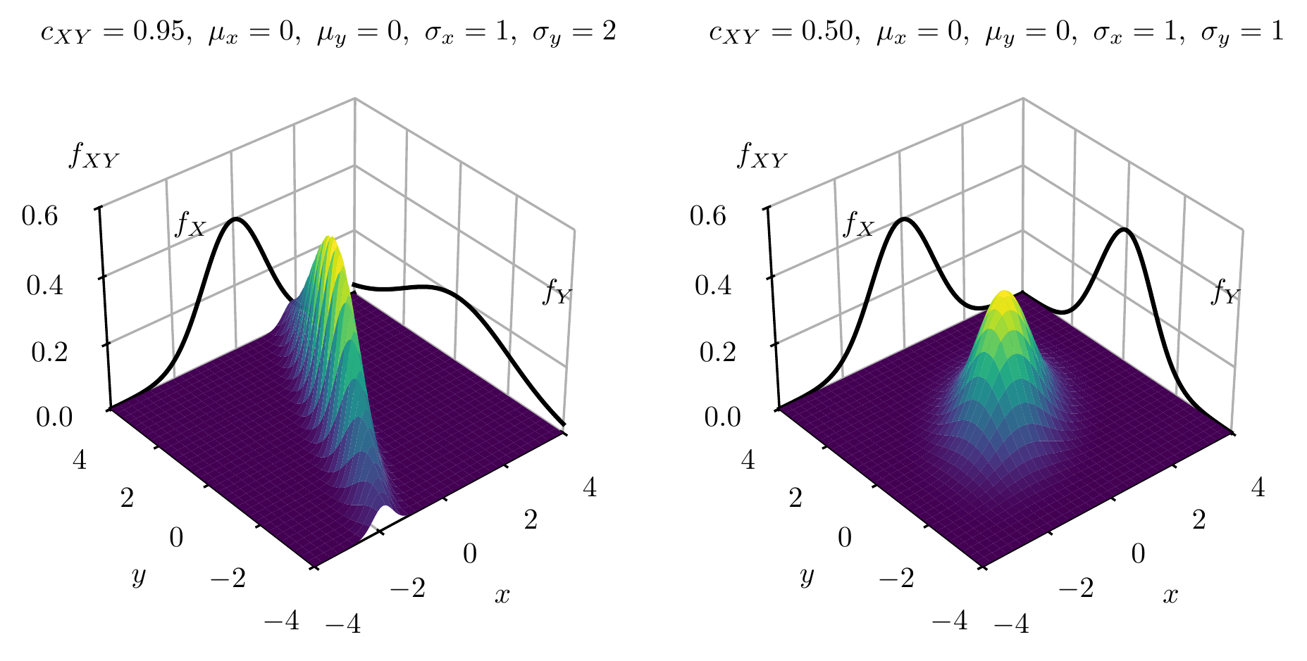
Which of the following statements are correct?
- The marginal density f_X(x) is obtained by integrating the joint density over all values of Y: f_X(x) = \int_{-\infty}^{\infty} f_{XY}(x, \eta) \, d\eta
- The joint PDF satisfies \int_{-\infty}^{\infty}\!\int_{-\infty}^{\infty} f_{XY}(x,y)\,dx\,dy = 1
- If we know f_X(x) and f_Y(y) individually, we can always reconstruct f_{XY}(x, y) as f_X(x) \cdot f_Y(y)
- Marginal densities always have the same shape as the joint density
- The joint density f_{XY}(x,y) is obtained from the joint CDF by partial differentiation: f_{XY}(x,y) = \frac{\partial^2 F_{XY}}{\partial x \,\partial y}
- ✓ Correct. Marginalization “integrates out” the variable we are not interested in, projecting the joint density onto the remaining variable.
- ✓ Correct. The total probability over the entire xy-plane must equal 1, just as for the one-dimensional case.
- ✗ Incorrect. The factorization f_{XY}(x,y) = f_X(x) f_Y(y) holds only when X and Y are statistically independent. In general, the joint PDF encodes dependence information that cannot be recovered from the marginals alone.
- ✗ Incorrect. Marginalization fundamentally changes the shape. For example, a bimodal joint density might produce unimodal marginals, and the spread of the marginal depends on the correlation structure. The marginal is a “projection,” not a “slice.”
- ✓ Correct. This is the two-dimensional generalization of f_X(x) = dF_X(x)/dx.
Correct: Marginalization integrates out unwanted variables from the joint density. The joint PDF normalizes to 1 over the full space and is obtained by differentiating the joint CDF. The marginals alone cannot reconstruct the joint density unless independence holds.
Review: Review the key distinction: knowing the marginals f_X and f_Y separately is not enough to know f_{XY} unless the variables are independent. Marginalization is integration, not restriction.
Q020 Statistical Independence of Random Variables
Understanding what independence means for the joint distribution and density of RVs
Which of the following statements about statistical independence of two random variables X and Y are correct?
- Independence requires that F_{XY}(x,y) = F_X(x) \cdot F_Y(y) for all x, y \in \mathbb{R}
- If X and Y are independent, then f_{X|Y}(x|y) = f_X(x), meaning knowledge of Y does not change the distribution of X
- If f_{XY}(x_0, y_0) = f_X(x_0) \cdot f_Y(y_0) holds at one particular point (x_0, y_0), then X and Y are independent
- For the joint distribution of independent RVs, the joint density is completely determined by the marginal densities
- Two RVs that are uncorrelated (zero covariance) are always independent
- ✓ Correct. This is the definition of statistical independence for RVs — the joint CDF factorizes into the product of marginal CDFs for all x and y.
- ✓ Correct. Under independence, f_{XY}(x,y) = f_X(x) f_Y(y), so f_{X|Y}(x|y) = f_{XY}(x,y)/f_Y(y) = f_X(x).
- ✗ Incorrect. Independence requires the factorization to hold for all (x, y), not just at a single point. A coincidental match at one point does not establish independence.
- ✓ Correct. When X and Y are independent, f_{XY}(x,y) = f_X(x) f_Y(y), so the marginals fully determine the joint density.
- ✗ Incorrect. Uncorrelatedness means \text{Cov}(X,Y) = 0, which is a weaker condition than independence. There exist uncorrelated RVs that are dependent — independence implies uncorrelatedness but not vice versa.
Correct: Independence of RVs means complete factorization of the joint distribution into marginals — at every point, not just some. It also implies that conditioning on one variable does not alter the distribution of the other. Independence is strictly stronger than uncorrelatedness.
Review: Remember that independence is defined by the factorization F_{XY} = F_X \cdot F_Y holding everywhere. A single matching point is not sufficient. Also review the relationship: independence \Rightarrow uncorrelatedness, but not the reverse.
Q021 Conditional Distributions and Densities
Understanding how conditioning on an event changes the distribution of an RV
Which of the following statements about conditional distributions and densities are correct?
Consider a uniformly distributed RV X on [0, x_{\max}] and the event A = \{x_{\max}/4 < X \leq x_{\max}/2\}.
- The conditional CDF is F_{X|A}(x) = \mathbb{P}(X \leq x \,|\, A) = \frac{\mathbb{P}(X \leq x \cap A)}{\mathbb{P}(A)}
- The conditional PDF f_{X|A}(x) is obtained by differentiating F_{X|A}(x) with respect to x
- For this example, the conditional PDF satisfies f_{X|A}(x) = 4 \cdot f_X(x) within the interval (x_{\max}/4, x_{\max}/2] and is zero elsewhere
- Conditioning on event A effectively restricts the sample space and renormalizes the density to integrate to 1
- The conditional density f_{X|A}(x) will have a lower peak than the unconditional f_X(x) because we are restricting to fewer outcomes
- ✓ Correct. This follows directly from the definition of conditional probability applied to the event \{X \leq x\} given A.
- ✓ Correct. As with any CDF-to-PDF relationship, f_{X|A}(x) = dF_{X|A}(x)/dx.
- ✓ Correct. Since \mathbb{P}(A) = 1/4 for a uniform distribution, conditioning “rescales” the PDF by 1/\mathbb{P}(A) = 4 within the conditioning interval and sets it to zero outside.
- ✓ Correct. Conditioning restricts attention to outcomes within A and rescales probabilities so that the conditional density integrates to 1 over the restricted domain.
- ✗ Incorrect. The conditional density actually has a higher peak. Since the probability mass is concentrated into a smaller interval but must still integrate to 1, the density increases. In this example, f_{X|A}(x) = 4 f_X(x) within the interval.
Correct: Conditioning restricts the distribution to a subset of outcomes and renormalizes the density. The conditional PDF is higher (more concentrated) than the original over the restricted interval, because the same normalization (total probability 1) is spread over a smaller domain.
Review: Think about area: the conditional PDF must integrate to 1 over a smaller interval. If the interval is smaller, the density must be taller to maintain unit area.
Q022 Conditional Density for Continuous RVs
Understanding conditional densities when conditioning on continuous random variables
Which of the following statements about the conditional density f_{X|Y}(x|y) for continuous random variables are correct?
- The conditional density is defined via the factorization f_{XY}(x,y) = f_{X|Y}(x|y) \cdot f_Y(y)
- For a continuous RV Y, the conditional density f_{X|Y}(x|y) is computed as f_{X|Y}(x|y) = \frac{f_{XY}(x,y)}{f_Y(y)} whenever f_Y(y) > 0
- Conditioning on the event \{Y = y\} for a continuous RV is done by computing \mathbb{P}(X \leq x \cap Y = y) / \mathbb{P}(Y = y)
- If X and Y are independent, then f_{X|Y}(x|y) = f_X(x) — the conditional density reduces to the marginal density
- The conditional density f_{X|Y}(x|y) does not need to integrate to 1 over x for a given y
- ✓ Correct. This is the defining relationship. It mirrors the event-level rule \mathbb{P}(A \cap B) = \mathbb{P}(A|B) \mathbb{P}(B) but at the density level.
- ✓ Correct. Dividing both sides of the factorization by f_Y(y) gives the conditional density, valid wherever the marginal density is positive.
- ✗ Incorrect. For a continuous RV, \mathbb{P}(Y = y) = 0, so this ratio is undefined (0/0). The conditional density is instead defined via the factorization of the joint density, avoiding the division by zero.
- ✓ Correct. Under independence, f_{XY}(x,y) = f_X(x)f_Y(y), so f_{X|Y}(x|y) = f_X(x)f_Y(y)/f_Y(y) = f_X(x).
- ✗ Incorrect. For any fixed y with f_Y(y) > 0, f_{X|Y}(x|y) is a valid density in x and must satisfy \int_{-\infty}^{\infty} f_{X|Y}(x|y)\,dx = 1.
Correct: The conditional density for continuous RVs avoids the \mathbb{P}(Y = y) = 0 issue by working directly with the density factorization. For any fixed y where f_Y(y) > 0, the conditional density is a proper PDF in x (integrates to 1). Independence makes the conditional density equal to the marginal.
Review: For continuous RVs, \mathbb{P}(Y = y) = 0, so conditioning cannot be defined as a ratio of probabilities. Instead, the conditional density is defined through the joint and marginal densities. Also remember that a conditional density is still a proper PDF.
Ch 3 — Stochastic Processes
§ 3.1 Definition
Q056 Definition of a Stochastic Process
Understanding the dual interpretation of a stochastic process as a function of both outcome and time index
Which of the following statements about the definition of a stochastic process are correct?
A stochastic process X[\eta, k] is a two-parameter function: \eta \in H (sample space) and k (discrete time index).
- A stochastic process X[\eta, k] maps each outcome \eta to an entire sequence indexed by k, called a sample function (realization)
- For a fixed outcome \eta_0, X[\eta_0, k] is a deterministic sequence — the sample function or realization associated with that outcome
- For a fixed time index k_0, X[\eta, k_0] is a random variable — its value depends on the random outcome \eta
- A stochastic process is simply a single random variable observed repeatedly at different times
- All sample functions of a stochastic process must share the same waveform shape, differing only in amplitude
- ✓ Correct. For a fixed outcome \eta, the stochastic process yields a deterministic sequence x[k] = X[\eta, k], which is a single realization or sample function.
- ✓ Correct. Fixing \eta removes the randomness; the result is one particular time series x[k].
- ✓ Correct. At each time instant k_0, the stochastic process defines a random variable over the sample space H.
- ✗ Incorrect. At each time index k, a stochastic process defines a (potentially different) random variable. The collection of all these random variables — with their joint distributions — constitutes the process.
- ✗ Incorrect. Sample functions can differ arbitrarily in shape, amplitude, and behavior. The only constraint is that they are drawn according to the underlying probability law.
Correct: A stochastic process has a dual interpretation: fix \eta to get a deterministic time series (sample function), or fix k to get a random variable. The ensemble of all sample functions, together with their probability structure, fully characterizes the process.
Review: Review the two-parameter interpretation of X[\eta, k]. Think carefully about what happens when you fix one argument and vary the other.
Q064 Examples of Stochastic Processes
Stationarity and ergodicity of AR(1), Pólya urn, and geometric random walk processes
Which of the following statements about common stochastic process examples are correct?
Consider the following processes: - AR(1): X[k] = a \cdot X[k-1] + W[k] with |a| < 1 and W[k] i.i.d. white noise - Pólya urn: draw a ball, return it with an extra ball of the same color - Geometric random walk: X[k] = \prod_{i=1}^{k} Z_i where Z_i are i.i.d. positive random variables
The figure shows several realizations of an AR(1) process.
- The AR(1) process with |a| < 1 and i.i.d. white noise input is WSS and ergodic (after reaching steady state)
- The Pólya urn process is NOT stationary because the composition of the urn — and thus the probability of drawing each color — changes over time
- A geometric random walk X[k] = \prod_{i=1}^{k} Z_i with i.i.d. factors is generally not WSS, because its variance grows (or shrinks) with k
- An AR(1) process with |a| > 1 is stable and WSS
- The Pólya urn process always converges to a uniform distribution over the colors
- ✓ Correct. For |a| < 1 the AR(1) process is stable, and its steady-state distribution has constant mean and a lag-dependent ACF R_{XX}[\kappa] = \frac{\sigma_W^2}{1 - a^2} a^{|\kappa|}. It is also ergodic.
- ✓ Correct. As balls are added, the distribution of outcomes evolves, making the process non-stationary.
- ✓ Correct. Even if \mathbb{E}[Z_i] = 1, the variance \text{Var}(X[k]) depends on k, violating the constant-ACF requirement of WSS.
- ✗ Incorrect. When |a| > 1, the AR(1) recursion is unstable — the variance of X[k] grows without bound, so the process is neither stable nor WSS.
- ✗ Incorrect. The limiting proportion of colors in a Pólya urn follows a Beta distribution (for two colors) and is random, not deterministically uniform. Different realizations converge to different proportions.
Correct: The AR(1) process is a fundamental building block in signal processing and time-series analysis: stable (|a|<1), WSS, and ergodic. The Pólya urn and geometric random walk illustrate non-stationary behavior arising from evolving distributions and multiplicative dynamics, respectively.
Review: Review the stability condition |a| < 1 for AR(1) and why it matters for stationarity. For the Pólya urn, think about how the composition changes after each draw. For the geometric random walk, compute the variance as a function of k.
§ 3.2–3.3 Expected Values
Q057 Autocorrelation and Autocovariance Properties
Properties of the autocorrelation function (ACF) and autocovariance function (ACV)
Which of the following statements about the autocorrelation function (ACF) and autocovariance function (ACV) of a stochastic process are correct?
- The ACF is defined as R_{XX}[k_1, k_2] = \mathbb{E}[X[k_1]\, X^*[k_2]]
- For a WSS process, R_{XX}[0] \geq |R_{XX}[\kappa]| for all lags \kappa — the ACF attains its maximum at zero lag
- For a WSS process, R_{XX}[-\kappa] = R_{XX}^*[\kappa] (conjugate symmetry)
- The ACF R_{XX}[\kappa] is always non-negative for all lags \kappa
- The ACF of a WSS process can grow without bound as the lag |\kappa| increases
- ✓ Correct. This is the standard definition of the autocorrelation function as the expected value of the product of the process at two time indices.
- ✓ Correct. This follows from the Cauchy–Schwarz inequality applied to the random variables X[k] and X[k+\kappa].
- ✓ Correct. Swapping the time arguments conjugates the ACF, giving R_{XX}[-\kappa] = R_{XX}^*[\kappa]. For real-valued processes this simplifies to even symmetry.
- ✗ Incorrect. The ACF can take negative values. For example, the ACF of a cosine process R_{XX}[\kappa] = \frac{A^2}{2}\cos(\Omega_0 \kappa) takes negative values at certain lags.
- ✗ Incorrect. Since |R_{XX}[\kappa]| \leq R_{XX}[0] for all \kappa, the ACF is bounded by its value at zero lag.
Correct: The ACF captures second-order temporal dependencies. Key properties for WSS processes include: maximum at zero lag, conjugate symmetry, and the relationship to the ACV via C_{XX}[\kappa] = R_{XX}[\kappa] - |m_X|^2.
Review: Review the definition of ACF and its fundamental properties. Remember that R_{XX}[0] = \mathbb{E}[|X[k]|^2] represents the average power, and the Cauchy–Schwarz inequality constrains the ACF at nonzero lags.
Q063 Cross-Correlation and Cross-Covariance
Properties of cross-correlation and cross-covariance functions between two processes
Which of the following statements about the cross-correlation function (CCF) and cross-covariance function (CCV) of two stochastic processes X[k] and Y[k] are correct?
- The CCF is defined as R_{XY}[k_1, k_2] = \mathbb{E}[X[k_1]\, Y^*[k_2]]
- The CCV is obtained by removing the means: C_{XY}[k_1, k_2] = R_{XY}[k_1, k_2] - m_X[k_1]\, m_Y^*[k_2]
- For jointly WSS processes, R_{XY}[\kappa] = R_{YX}[\kappa] — the CCF is symmetric in the subscript order
- The CCF R_{XY}[\kappa] is always symmetric in the lag, i.e., R_{XY}[\kappa] = R_{XY}[-\kappa]
- For jointly WSS processes, |R_{XY}[\kappa]| is always bounded: |R_{XY}[\kappa]|^2 \leq R_{XX}[0] \cdot R_{YY}[0]
- ✓ Correct. This is the standard definition of the cross-correlation function between processes X and Y.
- ✓ Correct. The cross-covariance subtracts the product of means from the cross-correlation, isolating the correlated fluctuations.
- ✗ Incorrect. The correct symmetry relation is R_{XY}[\kappa] = R_{YX}^*[-\kappa]. Swapping X and Y reverses the lag and conjugates the result.
- ✗ Incorrect. Unlike the ACF, the CCF is generally not symmetric in \kappa. The symmetry property involves both lag reversal and conjugation: R_{XY}[\kappa] = R_{YX}^*[-\kappa].
- ✓ Correct. This follows from the Cauchy–Schwarz inequality applied to X[k] and Y[k+\kappa]. The bound says the cross-correlation magnitude cannot exceed the geometric mean of the individual average powers.
Correct: The CCF and CCV characterize the linear relationship between two processes at different time lags. For jointly WSS processes, the CCF depends only on the lag \kappa, but unlike the ACF, it lacks even symmetry. The key symmetry relation is R_{XY}[\kappa] = R_{YX}^*[-\kappa].
Review: Review the definitions of CCF and CCV, and pay attention to the order of subscripts. Remember that cross-correlation does not have the same symmetry properties as autocorrelation.
Q065 Time Averages: Energy and Power
Definitions and properties of signal energy, average power, and their relation to ensemble averages
Which of the following statements about time-domain energy and power of signals and stochastic processes are correct?
- Total energy of a deterministic signal is E_x = \sum_{k=-\infty}^{\infty} |x[k]|^2, and average power is P_x = \lim_{N\to\infty} \frac{1}{2N+1}\sum_{k=-N}^{N} |x[k]|^2
- For an ergodic WSS process, the time-averaged power equals the ensemble average power: P_x = R_{XX}[0] = \mathbb{E}[|X[k]|^2]
- Every signal has finite total energy
- Power signals have finite energy
- The time average \langle x[k] \rangle = \lim_{N\to\infty}\frac{1}{2N+1}\sum_{k=-N}^{N} x[k] always equals \mathbb{E}[X[k]] for any WSS process
- ✓ Correct. These are the standard definitions of total energy and average power for discrete-time signals.
- ✓ Correct. Ergodicity ensures that the time average of |x[k]|^2 over a single realization converges to the ensemble second moment R_{XX}[0].
- ✗ Incorrect. Signals with nonzero average power (power signals) have infinite total energy. For example, a constant nonzero signal or a periodic signal has E_x = \infty.
- ✗ Incorrect. A power signal is defined as having finite nonzero average power, which implies infinite total energy. Energy signals and power signals are mutually exclusive categories.
- ✗ Incorrect. The time average equals the ensemble mean only for ergodic processes. A WSS but non-ergodic process (e.g., X[k]=C) has a time average that is random and generally differs from \mathbb{E}[X[k]].
Correct: The distinction between energy and power signals is fundamental: energy signals have finite total energy and zero average power, while power signals have infinite energy but finite nonzero average power. For ergodic WSS processes, time averages provide consistent estimates of ensemble statistics.
Review: Review the definitions of energy and power signals and why they are mutually exclusive. Remember that the equality of time and ensemble averages requires ergodicity, not just stationarity.
§ 3.4 Properties of Random Processes
Q060 Gaussian Processes
Special properties of Gaussian stochastic processes
Which of the following statements about Gaussian stochastic processes are correct?
- A Gaussian process is one in which any finite collection of samples (X[k_1], X[k_2], \ldots, X[k_N]) is jointly Gaussian
- For a Gaussian WSS process, uncorrelated samples are also statistically independent — so a Gaussian weak-sense white noise process is strict-sense white
- For Gaussian processes, WSS implies SSS, because Gaussian distributions are completely characterized by their mean vector and covariance matrix
- A process is Gaussian if each individual sample X[k] has a Gaussian marginal distribution
- Marginal Gaussianity of each X[k] implies joint Gaussianity of the process
- ✓ Correct. The defining property of a Gaussian process is that all finite-dimensional distributions are multivariate Gaussian.
- ✓ Correct. For jointly Gaussian random variables, uncorrelatedness implies independence. Therefore Gaussian weak-sense white noise is automatically strict-sense white.
- ✓ Correct. Since a Gaussian distribution is fully specified by its first two moments, the WSS conditions (constant mean, lag-only ACF) fix all joint distributions, yielding SSS.
- ✗ Incorrect. Marginally Gaussian samples do not guarantee a jointly Gaussian process. The defining requirement is that all finite-dimensional joint distributions are Gaussian.
- ✗ Incorrect. It is possible to construct random variables that are each marginally Gaussian but whose joint distribution is not Gaussian. Joint Gaussianity is a stronger condition.
Correct: Gaussian processes occupy a special place in the theory of stochastic processes: their full statistical description is determined by the mean function and autocovariance. This makes WSS equivalent to SSS and uncorrelatedness equivalent to independence — simplifications that do not hold for general processes.
Review: Review the distinction between marginal and joint distributions. Remember that a Gaussian process requires all finite-dimensional distributions to be jointly Gaussian, which is stronger than requiring each sample to be individually Gaussian.
§ 3.5 Stationarity
Q058 Wide-Sense vs. Strict-Sense Stationarity
Distinguishing between WSS and SSS and understanding their relationship
Which of the following statements about wide-sense stationarity (WSS) and strict-sense stationarity (SSS) are correct?
- WSS requires two conditions: constant mean m_X[k] = m_X and an ACF that depends only on the lag \kappa = k_1 - k_2, i.e., R_{XX}[k_1, k_2] = R_{XX}[\kappa]
- SSS requires that all joint distributions f_{X[k_1], \ldots, X[k_N]} are invariant under arbitrary time shifts
- WSS implies SSS for any stochastic process
- WSS requires all moments (not just first and second) to be shift-invariant
- SSS and WSS are completely equivalent definitions of stationarity
- ✓ Correct. WSS constrains only the first two moments: the mean must be time-invariant and the ACF must be a function of lag alone.
- ✓ Correct. Strict-sense stationarity means every finite-dimensional distribution is unchanged when all time indices are shifted by the same amount.
- ✗ Incorrect. WSS constrains only the first two moments, not the full distribution. A WSS process can have higher-order statistics that vary with time, so WSS does not imply SSS in general. (The exception is Gaussian processes, where the distribution is fully determined by mean and covariance.)
- ✗ Incorrect. WSS only constrains the mean (first moment) and the autocorrelation (second moment). Higher-order moments are unrestricted.
- ✗ Incorrect. SSS is strictly stronger than WSS. Every SSS process (with finite second moments) is WSS, but the converse does not hold in general.
Correct: WSS is a practical, second-order characterization: constant mean and lag-dependent ACF. SSS is the full statistical characterization requiring shift-invariance of all joint distributions. SSS implies WSS (given finite second moments), but WSS does not imply SSS unless additional structure (e.g., Gaussianity) is present.
Review: Carefully distinguish which statistical properties each type of stationarity constrains. WSS involves only the first two moments, while SSS involves the entire probability structure.
Q059 White Noise
Properties of weak-sense and strict-sense white noise processes
Which of the following statements about white noise processes are correct?
- Weak-sense white noise has an autocovariance of the form C_{XX}[k_1, k_2] = C_0\, \delta[k_1 - k_2], meaning distinct samples are uncorrelated
- Strict-sense white noise requires that X[k_1] and X[k_2] are statistically independent for k_1 \neq k_2
- White noise must be Gaussian-distributed
- Weak-sense white noise means that distinct samples are statistically independent
- White noise has zero average power
- ✓ Correct. Weak-sense white noise is defined by the property that samples at different time indices are uncorrelated, with all covariance concentrated at zero lag.
- ✓ Correct. Strict-sense white noise strengthens the condition from uncorrelatedness to full statistical independence of distinct samples.
- ✗ Incorrect. White noise can have any marginal distribution. “White” refers to the spectral/correlation property (uncorrelated or independent samples), not to the amplitude distribution.
- ✗ Incorrect. Weak-sense white requires only uncorrelatedness (C_{XX}[k_1,k_2]=0 for k_1 \neq k_2). Independence is a stronger condition that defines strict-sense white noise.
- ✗ Incorrect. The average power of white noise is R_{XX}[0] = \mathbb{E}[|X[k]|^2], which equals the variance plus the squared mean. This is generally nonzero.
Correct: White noise is characterized by the absence of temporal correlation. Weak-sense white noise requires uncorrelated samples; strict-sense white noise requires independent samples. The term “white” comes from the flat (constant) power spectral density, analogous to white light containing all frequencies equally.
Review: Review the distinction between uncorrelatedness (second-order property) and independence (full distributional property). Remember that “white” describes the spectral shape, not the amplitude distribution.
Q062 Cosine Process with Random Phase
Stationarity and ergodicity of the random-phase cosine process
Which of the following statements about the process X[k] = A\cos(\Omega_0 k + \Phi) are correct?
Assume A and \Omega_0 are deterministic constants and \Phi is a random variable uniformly distributed on [0, 2\pi).
- The process X[k] = A\cos(\Omega_0 k + \Phi) with \Phi \sim \mathcal{U}[0, 2\pi) is wide-sense stationary
- The mean of X[k] is zero: m_X = \mathbb{E}[A\cos(\Omega_0 k + \Phi)] = 0
- The ACF depends only on the lag: R_{XX}[\kappa] = \frac{A^2}{2}\cos(\Omega_0 \kappa)
- This process is also ergodic: time averages of any single realization converge to the ensemble averages
- The process X[k] = A\cos(\Omega_0 k + \phi_0) with a deterministic (fixed) phase \phi_0 is also WSS
- ✓ Correct. The uniform phase ensures that the mean is zero and the ACF depends only on the lag \kappa, satisfying both WSS conditions.
- ✓ Correct. Integrating \cos(\Omega_0 k + \phi) over a full period \phi \in [0, 2\pi) with uniform weight yields zero.
- ✓ Correct. Using the product-to-sum formula and averaging over \Phi eliminates dependence on absolute time, leaving R_{XX}[\kappa] = \frac{A^2}{2}\cos(\Omega_0 \kappa).
- ✓ Correct. For a single realization (fixed \Phi), the time average of \cos(\Omega_0 k + \Phi) over increasing intervals converges to zero (the ensemble mean), and similarly for the time-averaged ACF.
- ✗ Incorrect. With a fixed phase, X[k] is a deterministic signal — there is no randomness. It does not satisfy the WSS definition because there is no ensemble to average over (or equivalently, the “mean” m_X[k] = A\cos(\Omega_0 k + \phi_0) depends on k).
Correct: The random-phase cosine is a classic example of a WSS and ergodic process. The key is that the uniform phase \Phi randomizes the process enough to make the mean constant (zero) and the ACF lag-dependent. Without the random phase, the signal is deterministic and not stationary.
Review: Review why the uniform distribution of \Phi over [0, 2\pi) is essential for stationarity. Compute the mean and ACF explicitly, and notice how a fixed phase breaks the time-invariance of the mean.
Q066 Barker Sequences
Autocorrelation properties and applications of Barker sequences
Which of the following statements about Barker sequences are correct?
A Barker sequence is a finite binary sequence \{a_n\} with a_n \in \{-1, +1\} that has special autocorrelation properties.
- Barker sequences have the property that all off-peak (sidelobe) autocorrelation values have magnitude at most 1
- Barker sequences are used in radar and communications for pulse compression, enabling sharp range resolution
- Barker sequences exist for any desired length N
- The autocorrelation sidelobes of a Barker sequence are always exactly zero
- Barker sequences are only useful in the presence of Gaussian noise
- ✓ Correct. The defining property of a Barker sequence of length N is that |R[k]| \leq 1 for all k \neq 0, where R[k] is the aperiodic autocorrelation.
- ✓ Correct. The low sidelobe property allows transmitted pulses to be compressed upon reception, improving range resolution while maintaining energy efficiency.
- ✗ Incorrect. Barker sequences are known to exist only for very few lengths (N = 2, 3, 4, 5, 7, 11, 13). It has been conjectured that no Barker sequences exist for N > 13.
- ✗ Incorrect. The sidelobes have magnitude at most 1, not exactly zero. A sequence with exactly zero sidelobes would be an ideal thumbtack autocorrelation, which does not exist for finite-length binary sequences.
- ✗ Incorrect. The low-sidelobe autocorrelation property is valuable regardless of the noise distribution. Barker sequences are useful for detection, synchronization, and ranging in diverse noise environments.
Correct: Barker sequences provide near-ideal autocorrelation properties for finite binary sequences: a sharp peak at zero lag with all sidelobes bounded by 1 in magnitude. Their rarity (only lengths up to 13 are known) makes them particularly valued in radar and communication system design.
Review: Review the definition of Barker sequences and their autocorrelation properties. Remember that the sidelobe bound is |R[k]| \leq 1, not R[k] = 0, and that only finitely many Barker lengths are known.
§ 3.6 Ergodicity
Q061 Ergodicity
Understanding ergodicity and the relationship between time and ensemble averages
Which of the following statements about ergodicity of stochastic processes are correct?
- An ergodic process is one for which time averages converge to the corresponding ensemble averages with probability 1
- A constant process X[k] = C, where C is a non-degenerate random variable, is NOT ergodic: the time average of any realization equals C, which is random and generally does not equal \mathbb{E}[C] with probability 1
- All WSS processes are ergodic
- Ergodicity guarantees that statistics estimated from a single realization are always exact, regardless of the realization length
- Non-stationary processes can be ergodic
- ✓ Correct. Ergodicity means that statistical properties (mean, correlation, etc.) can be determined from a single, sufficiently long realization, because time averages equal ensemble averages almost surely.
- ✓ Correct. Each realization is a constant sequence with value C, so the time average is C itself — a random variable, not the deterministic ensemble mean \mathbb{E}[C].
- ✗ Incorrect. WSS is necessary but not sufficient for ergodicity. The constant process X[k] = C is WSS but not ergodic, providing a direct counterexample.
- ✗ Incorrect. Ergodicity guarantees convergence of time averages to ensemble averages in the limit of infinite observation length. For any finite realization, the estimates are approximations subject to estimation error.
- ✗ Incorrect. Ergodicity requires stationarity as a prerequisite. A non-stationary process has time-varying statistics, making it impossible for a single time average to represent the (non-constant) ensemble average.
Correct: Ergodicity bridges the gap between theoretical ensemble averages and practical time-domain measurements. It requires stationarity and an additional “mixing” condition ensuring that the process explores its full statistical range over time. The constant process is a classic counterexample: WSS but not ergodic.
Review: Review the definition of ergodicity and why stationarity alone is not sufficient. Consider what happens when you try to estimate the mean of a constant process from a single realization.
Q067 Ensemble Averages vs. Time Averages
Understanding the fundamental distinction between ensemble and time averages
Which of the following statements about ensemble averages and time averages of stochastic processes are correct?
- The ensemble average at time k_0 is computed by averaging X[\eta, k_0] across all realizations \eta: \mathbb{E}[X[k_0]] = \int X[\eta, k_0]\, d\mathbb{P}(\eta)
- The time average for a fixed realization \eta_0 is computed by averaging X[\eta_0, k] across time: \langle x[k] \rangle = \lim_{N\to\infty}\frac{1}{2N+1}\sum_{k=-N}^{N} X[\eta_0, k]
- For ergodic processes, ensemble averages and time averages converge to the same value (with probability 1)
- Ensemble averages and time averages are always equal for any stochastic process
- Computing a time average requires access to multiple independent realizations of the process
- ✓ Correct. The ensemble average fixes the time index and averages over the probability space — it is a statistical (expectation) operation.
- ✓ Correct. The time average fixes the realization and averages over the time index — it is a temporal operation on a single sample function.
- ✓ Correct. This is precisely the defining property of ergodicity: time averages computed from a single realization equal the ensemble (statistical) averages almost surely.
- ✗ Incorrect. Equality of ensemble and time averages holds only for ergodic processes. For non-ergodic processes (e.g., X[k] = C with random C), the time average is C (random) while the ensemble average is \mathbb{E}[C] (deterministic).
- ✗ Incorrect. A time average is computed from a single realization by averaging along the time axis. It is the ensemble average that conceptually requires multiple realizations (or knowledge of the probability distribution).
Correct: The distinction between ensemble and time averages is central to the practical application of stochastic process theory. Ensemble averages are theoretical expectations; time averages are what we can compute from measured data. Ergodicity is the bridge that justifies using one for the other.
Review: Review the definitions: ensemble average fixes time and averages over realizations; time average fixes a realization and averages over time. Think about when and why these two quantities coincide.
Q068 The Constant Process
Stationarity and ergodicity of the constant random process X[k] = C
Which of the following statements about the constant process X[k] = C are correct?
Here C is a random variable with \mathbb{E}[C] = \mu and \text{Var}\{C\} = \sigma^2 > 0.
- The constant process X[k] = C is WSS but NOT ergodic
- The process is ergodic because its mean and ACF do not depend on time
- The process is not WSS because R_{XX}[k_1, k_2] = \mathbb{E}[C^2] does not decay with lag
- The time average of any realization equals \mu
- The ACF of the constant process is zero for all lags
- ✓ Correct. It is WSS because m_X[k] = \mu (constant) and R_{XX}[k_1,k_2] = \mathbb{E}[C^2] depends only on the lag (trivially, since it is the same for all k_1, k_2). However, it is not ergodic because the time average of any realization equals C (random), not \mu (deterministic).
- ✗ Incorrect. Time-independent mean and ACF make the process WSS, not ergodic. Ergodicity additionally requires that time averages converge to ensemble averages — which fails here because the time average equals C, a random variable.
- ✗ Incorrect. WSS requires only that the ACF depends on the lag \kappa = k_1 - k_2, not that it decays. Here R_{XX}[\kappa] = \mathbb{E}[C^2] for all \kappa, which trivially satisfies the lag-only condition.
- ✗ Incorrect. Each realization is the constant sequence x[k] = c for some fixed value c drawn from C. The time average is c itself, not \mu = \mathbb{E}[C]. This mismatch between time average (C) and ensemble mean (\mu) is exactly why the process fails to be ergodic.
- ✗ Incorrect. The ACF is R_{XX}[\kappa] = \mathbb{E}[C \cdot C^*] = \mathbb{E}[|C|^2] = \mu^2 + \sigma^2 > 0 for all lags.
Correct: The constant process is the canonical example showing that WSS does not imply ergodicity. Every realization is “stuck” at one value of C, so a single realization reveals only one sample of C — no amount of time averaging can recover the full distribution.
Review: Carefully verify the WSS conditions (constant mean, lag-only ACF) and then check the ergodicity condition (time average = ensemble average a.s.). Compute the time average of a single realization x[k] = c and compare it with \mu.
§ 3.8 Power Spectral Density
Q069 Power Spectral Density (PSD) Definition
The Wiener–Khinchin theorem and fundamental properties of the PSD
Which of the following statements about the power spectral density (PSD) of a WSS process are correct?
- The PSD is the DTFT of the autocorrelation function (Wiener–Khinchin theorem): S_{XX}(e^{j\Omega}) = \sum_{\kappa=-\infty}^{\infty} R_{XX}[\kappa]\, e^{-j\Omega\kappa}
- The PSD is non-negative for all frequencies: S_{XX}(e^{j\Omega}) \geq 0 for all \Omega
- The total average power equals the integral of the PSD: R_{XX}[0] = \frac{1}{2\pi}\int_{-\pi}^{\pi} S_{XX}(e^{j\Omega})\, d\Omega
- The PSD can take negative values at certain frequencies
- The PSD is the Fourier transform of the probability density function (PDF) of X[k]
- ✓ Correct. The Wiener–Khinchin theorem establishes this Fourier-transform pair between the ACF and the PSD for WSS processes.
- ✓ Correct. The PSD represents the distribution of average power across frequency and must be non-negative, since it can be shown that the ACF is a positive semi-definite sequence.
- ✓ Correct. Setting \kappa = 0 in the inverse DTFT recovers R_{XX}[0] = \mathbb{E}[|X[k]|^2], the average power, as the normalized area under the PSD.
- ✗ Incorrect. The PSD is always non-negative. A negative PSD would imply negative power at some frequency, which is physically meaningless.
- ✗ Incorrect. The PSD is the DTFT of the autocorrelation function, not the PDF. The Fourier transform of a PDF is the characteristic function — a completely different concept.
Correct: The PSD provides a frequency-domain description of how a WSS process distributes its average power across frequencies. The Wiener–Khinchin theorem establishes the ACF \leftrightarrow PSD Fourier pair, and the non-negativity of the PSD is a fundamental constraint.
Review: Review the Wiener–Khinchin theorem and distinguish between the PSD (Fourier transform of ACF) and the characteristic function (Fourier transform of PDF). Remember that power cannot be negative, so neither can the PSD.
Q070 PSD of White Noise
Spectral properties of white noise processes
Which of the following statements about the power spectral density of white noise are correct?
Consider a WSS white noise process N[k] with zero mean and variance \sigma_N^2.
- The PSD of white noise is flat (constant): S_{NN}(e^{j\Omega}) = \sigma_N^2 for all \Omega
- The name “white” noise comes from the flat spectrum, by analogy with white light containing all visible frequencies equally
- White noise has a PSD that peaks at \Omega = 0 and decays toward \Omega = \pi
- White noise has infinite average power
- The PSD of white noise depends on frequency — different frequencies carry different amounts of power
- ✓ Correct. Since R_{NN}[\kappa] = \sigma_N^2 \delta[\kappa], the DTFT is the constant \sigma_N^2. All frequencies carry equal power.
- ✓ Correct. Just as white light is (approximately) a uniform mixture of all colors/frequencies, white noise has a uniform PSD.
- ✗ Incorrect. The PSD of white noise is constant (flat) across all frequencies. A spectrum that peaks at \Omega = 0 would characterize lowpass-filtered (colored) noise.
- ✗ Incorrect. For discrete-time white noise with finite variance \sigma_N^2, the average power is R_{NN}[0] = \sigma_N^2, which is finite. (Infinite power arises only in the continuous-time idealization with a flat PSD over an infinite bandwidth.)
- ✗ Incorrect. The defining spectral property of white noise is that its PSD is constant, meaning all frequencies carry the same power per unit bandwidth.
Correct: White noise is the simplest spectral model: a flat PSD at level \sigma_N^2 over all discrete-time frequencies \Omega \in [-\pi, \pi). This corresponds to an ACF that is a Kronecker delta, confirming that samples are uncorrelated.
Review: Review the DTFT of a Kronecker delta sequence. Remember that “white” means spectrally flat, and that discrete-time white noise with finite variance has finite average power \sigma_N^2.
Q071 Cross-Power Spectral Density and Coherence
Properties of the cross-PSD and the coherence function
Which of the following statements about the cross-power spectral density and coherence are correct?
- The cross-PSD is defined as the DTFT of the cross-correlation function: S_{XY}(e^{j\Omega}) = \sum_{\kappa=-\infty}^{\infty} R_{XY}[\kappa]\, e^{-j\Omega\kappa}
- The coherence function is defined as \gamma_{XY}(e^{j\Omega}) = \frac{S_{XY}(e^{j\Omega})}{\sqrt{S_{XX}(e^{j\Omega}) \cdot S_{YY}(e^{j\Omega})}}, with |\gamma_{XY}| \leq 1
- The cross-PSD S_{XY}(e^{j\Omega}) is always real-valued
- The cross-PSD S_{XY}(e^{j\Omega}) is always non-negative
- The magnitude of the coherence function can exceed 1 when the processes are strongly correlated
- ✓ Correct. For jointly WSS processes, the cross-PSD is the Fourier transform of the CCF, analogous to the Wiener–Khinchin theorem for the auto-PSD.
- ✓ Correct. The coherence is a normalized measure of linear frequency-domain association between two processes. Its magnitude is bounded by 1, analogous to the correlation coefficient.
- ✗ Incorrect. Unlike the auto-PSD, the cross-PSD is generally complex-valued because the CCF R_{XY}[\kappa] does not have even symmetry.
- ✗ Incorrect. Non-negativity holds for the auto-PSD S_{XX}, but the cross-PSD can be complex-valued and has no non-negativity constraint.
- ✗ Incorrect. By the Cauchy–Schwarz inequality, |\gamma_{XY}(e^{j\Omega})| \leq 1 always. A value of 1 indicates perfect linear relationship at that frequency; it cannot be exceeded.
Correct: The cross-PSD generalizes the PSD to pairs of processes and is generally complex-valued. The coherence function normalizes the cross-PSD to provide a frequency-by-frequency measure of linear dependence, bounded between 0 and 1 in magnitude.
Review: Review the differences between auto-PSD (real, non-negative) and cross-PSD (generally complex). Remember that coherence is bounded by 1 due to the Cauchy–Schwarz inequality.
Q074 Colored Noise
Generation and properties of colored (non-white) noise
Which of the following statements about colored noise are correct?
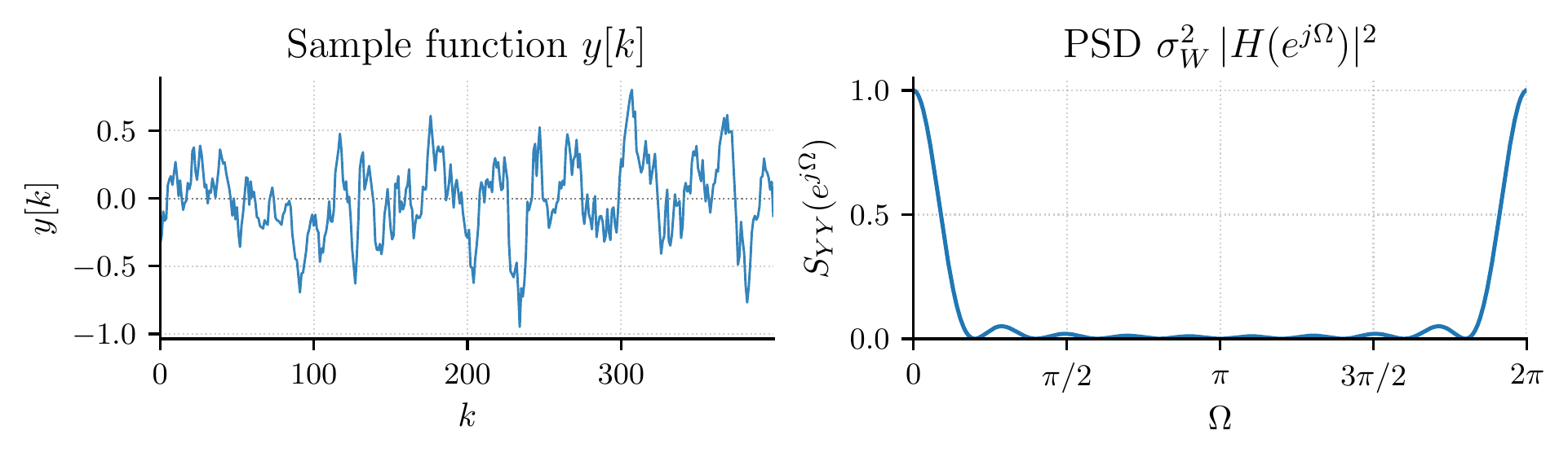
The figure illustrates a non-flat PSD characteristic of colored noise.
- Colored noise is a random process with a non-flat (frequency-dependent) power spectral density
- Colored noise can be generated by filtering white noise through an LTI system, yielding S_{YY}(e^{j\Omega}) = |H(e^{j\Omega})|^2 \sigma_W^2
- Colored noise is always non-stationary
- Colored noise has autocorrelation only at lag zero, like white noise
- All real-world noise is white noise
- ✓ Correct. Unlike white noise (flat PSD), colored noise has more power at some frequencies than others. The “color” metaphor refers to the spectral shape.
- ✓ Correct. Passing white noise (flat PSD \sigma_W^2) through an LTI filter with transfer function H shapes the spectrum by |H|^2, producing colored noise with the desired spectral profile.
- ✗ Incorrect. Colored noise can be perfectly stationary (WSS). “Colored” refers to the spectral shape, not to time-varying statistics. Filtering WSS white noise through a stable LTI system produces WSS colored noise.
- ✗ Incorrect. A non-flat PSD implies a non-impulsive ACF — colored noise samples are correlated across time. Only white noise has autocorrelation concentrated at zero lag.
- ✗ Incorrect. Most real-world noise sources (e.g., 1/f noise, thermal noise filtered by circuit bandwidth) have frequency-dependent PSDs and are therefore colored, not white.
Correct: Colored noise is a WSS process with a non-flat PSD, meaning its samples are temporally correlated. It arises naturally from filtering white noise through an LTI system or from physical processes with frequency-dependent characteristics.
Review: Review the distinction between “white” (flat PSD, uncorrelated samples) and “colored” (non-flat PSD, correlated samples). Remember that stationarity and spectral color are independent properties.
Q075 Parseval’s Relation and Average Power
Relating average power to the PSD via Parseval-like identities
Which of the following statements about average power and its spectral computation are correct?
- The average power of a WSS process equals the ACF at zero lag and the normalized integral of the PSD: R_{XX}[0] = \frac{1}{2\pi}\int_{-\pi}^{\pi} S_{XX}(e^{j\Omega})\, d\Omega
- For white noise with variance \sigma^2, the average power computed from the PSD is \frac{1}{2\pi}\int_{-\pi}^{\pi}\sigma^2\, d\Omega = \sigma^2
- The total average power is the area under the PSD divided by 2\pi, i.e., the PSD describes power density per unit frequency
- The average power is simply \int_{-\pi}^{\pi} S_{XX}(e^{j\Omega})\, d\Omega without the \frac{1}{2\pi} factor
- The PSD has units of energy, not power
- ✓ Correct. This is the inverse DTFT evaluated at \kappa=0, giving the Parseval-like power relation between time and frequency domains.
- ✓ Correct. The flat PSD \sigma^2 integrated over [-\pi, \pi) and divided by 2\pi gives exactly \sigma^2, consistent with R_{NN}[0] = \sigma^2.
- ✓ Correct. The PSD has units of power per radian/sample, so integrating over frequency and normalizing by 2\pi yields total average power.
- ✗ Incorrect. The \frac{1}{2\pi} normalization is essential in the inverse DTFT. Omitting it overestimates the power by a factor of 2\pi.
- ✗ Incorrect. The PSD describes the distribution of average power across frequency (power per unit frequency). Energy spectral density (ESD) is a different quantity that applies to deterministic finite-energy signals.
Correct: Parseval’s relation for stochastic processes connects the time-domain average power R_{XX}[0] to the frequency-domain integral of the PSD. The 1/(2\pi) normalization factor is a consequence of the DTFT convention and must not be forgotten.
Review: Review the inverse DTFT formula and set \kappa = 0 to derive the power relation. Pay attention to the 1/(2\pi) normalization factor and the distinction between PSD (power per frequency) and ESD (energy per frequency).
Q077 Energy Spectral Density
Energy spectral density for deterministic finite-energy signals and Parseval’s theorem
Which of the following statements about the energy spectral density (ESD) of deterministic finite-energy signals are correct?
- For a deterministic finite-energy signal x[k], the ESD is |X(e^{j\Omega})|^2, where X(e^{j\Omega}) is the DTFT of x[k]
- By Parseval’s theorem: E_x = \sum_{k=-\infty}^{\infty}|x[k]|^2 = \frac{1}{2\pi}\int_{-\pi}^{\pi}|X(e^{j\Omega})|^2\, d\Omega
- The ESD is always equal to the PSD
- A finite-energy signal has constant (nonzero) average power
- The ESD is the correct spectral description for random (stochastic) processes
- ✓ Correct. The ESD gives the distribution of signal energy across frequency for a deterministic signal with finite total energy.
- ✓ Correct. Parseval’s theorem equates total energy computed in the time domain (sum of squared magnitudes) with the frequency domain (normalized integral of the ESD).
- ✗ Incorrect. The ESD applies to deterministic finite-energy signals and measures energy per frequency. The PSD applies to random power signals and measures power per frequency. They are related but distinct concepts.
- ✗ Incorrect. A finite-energy signal has zero average power. The total energy is spread over infinite time, giving P_x = \lim_{N\to\infty}\frac{E_x}{2N+1} = 0.
- ✗ Incorrect. Stochastic processes with finite average power are described by the PSD (via the Wiener–Khinchin theorem), not the ESD. The ESD is used for deterministic, finite-energy signals.
Correct: The ESD and PSD are complementary spectral descriptions for different signal classes: ESD for deterministic finite-energy signals, PSD for stationary random processes. Parseval’s theorem connects time-domain energy to the integral of the ESD.
Review: Review the distinction between energy signals (finite energy, zero average power) and power signals (infinite energy, finite average power). Each class has its own spectral description: ESD and PSD, respectively.
Q078 Sinusoid Embedded in Noise
PSD and power of a sinusoidal signal corrupted by additive white noise
Which of the following statements about the process X[k] = A\cos(\Omega_0 k + \Phi) + N[k] are correct?
Assume \Phi \sim \mathcal{U}[0, 2\pi), N[k] is zero-mean white noise with variance \sigma_N^2, and the sinusoidal component and N[k] are independent.
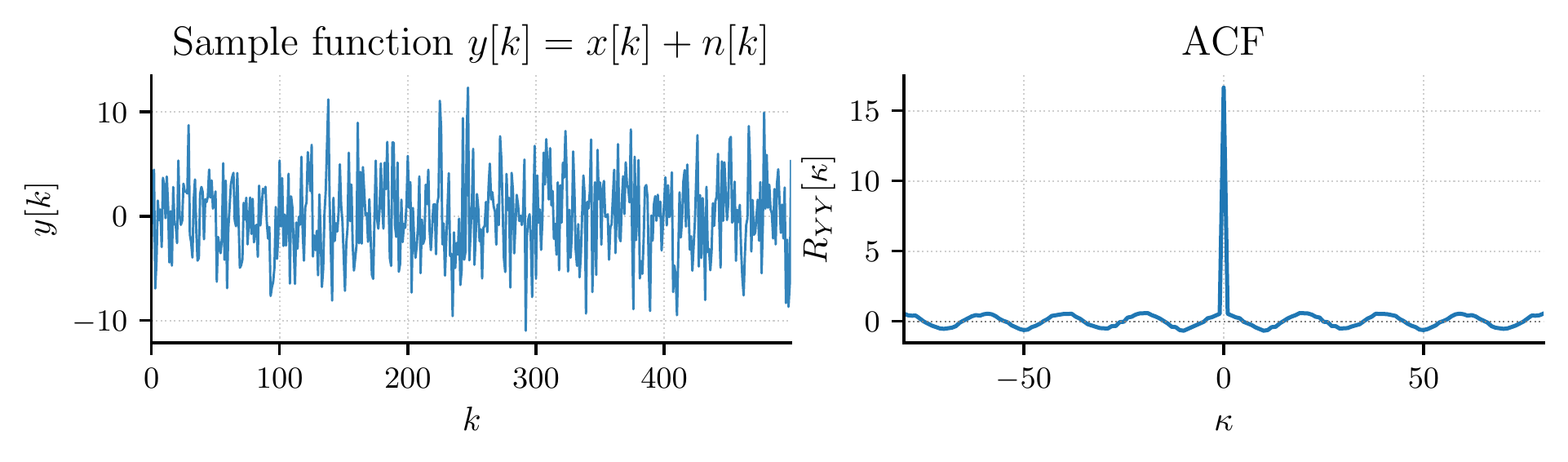
The figure illustrates a sinusoidal signal buried in additive noise.
- The PSD of X[k] contains Dirac impulses at \Omega = \pm\Omega_0 (from the sinusoid) plus a flat noise floor at level \sigma_N^2
- Since the signal and noise are independent and hence uncorrelated, their PSDs add: S_{XX} = S_{\text{signal}} + S_{\text{noise}}
- The total average power is P_X = \frac{A^2}{2} + \sigma_N^2
- The sinusoidal component has a continuous (spread-out) PSD, not Dirac impulses
- For independent signal and noise components, the PSDs multiply: S_{XX} = S_{\text{signal}} \cdot S_{\text{noise}}
- ✓ Correct. The sinusoidal component has PSD \frac{A^2}{4}\bigl[\delta(\Omega - \Omega_0) + \delta(\Omega + \Omega_0)\bigr] (scaled Dirac impulses), and the white noise contributes a constant \sigma_N^2. Since signal and noise are independent, their PSDs add.
- ✓ Correct. Independence implies zero cross-correlation, so R_{XX} = R_{\text{signal}} + R_{\text{noise}}. Taking the DTFT of both sides gives S_{XX} = S_{\text{signal}} + S_{\text{noise}}.
- ✓ Correct. The sinusoidal component contributes power A^2/2 and the noise contributes \sigma_N^2. By independence, total power is their sum.
- ✗ Incorrect. A pure sinusoid with random phase is a periodic power signal whose PSD consists of Dirac impulses at the signal frequency \pm\Omega_0, not a continuous spectrum.
- ✗ Incorrect. Independence causes the autocorrelation functions (and hence the PSDs) to add, not multiply. Multiplication of spectra arises in convolution scenarios, not in additive signal models.
Correct: A sinusoid in white noise is a classic signal detection scenario. The PSD has discrete spectral lines (Dirac impulses at \pm\Omega_0) rising above a flat noise floor. The total power is the sum of signal power (A^2/2) and noise power (\sigma_N^2), reflecting the additivity of PSDs for uncorrelated components.
Review: Review how PSDs combine for independent additive components (they add, not multiply). Remember that a periodic signal has a discrete (impulsive) PSD, not a continuous one.
§ 3.9 LTI Systems and WSS Processes
Q072 LTI Systems: Output Mean and Stationarity
Effect of an LTI system on the mean, stationarity, and PSD of a WSS input
Which of the following statements about the output of an LTI system driven by a WSS input are correct?
Let X[k] be a WSS input to an LTI system with impulse response h[k] and transfer function H(e^{j\Omega}). The output is Y[k] = \sum_n h[n]\, X[k-n].
- The output mean is m_Y = m_X \cdot H(e^{j0}) = m_X \cdot H(1), i.e., the input mean scaled by the DC gain
- The output Y[k] of an LTI system with WSS input is also WSS
- The output PSD is S_{YY}(e^{j\Omega}) = |H(e^{j\Omega})|^2 \cdot S_{XX}(e^{j\Omega})
- The output mean is m_Y = m_X \cdot |H(e^{j0})|^2
- The output of an LTI system with a WSS input is not necessarily WSS
- ✓ Correct. Taking the expectation of Y[k] = \sum_n h[n]\, X[k-n] and using the constant mean of X gives m_Y = m_X \sum_n h[n] = m_X \cdot H(e^{j0}).
- ✓ Correct. The constant mean of X maps to a constant mean of Y, and the lag-only ACF of X maps to a lag-only ACF of Y, preserving wide-sense stationarity.
- ✓ Correct. This fundamental result shows that the LTI system shapes the input PSD by the squared magnitude of the transfer function.
- ✗ Incorrect. The output mean involves H(e^{j0}) (the DC gain), not |H(e^{j0})|^2. The squared magnitude appears in the PSD relation, not the mean relation.
- ✗ Incorrect. A stable LTI system preserves wide-sense stationarity: if the input is WSS, the output is guaranteed to be WSS.
Correct: An LTI system preserves WSS and transforms the spectral content by |H|^2. The output mean is the input mean times the DC gain H(1). These results are the foundation for spectral analysis of filtered random signals.
Review: Review how the expectation operator interacts with the convolution sum. Distinguish between the DC gain H(e^{j0}) (which affects the mean) and the squared magnitude |H|^2 (which affects the PSD).
Q073 Output and Cross-PSD of LTI Systems
Detailed spectral input-output relations for LTI systems
Which of the following statements about the spectral input-output relations for an LTI system with transfer function H(e^{j\Omega}) and WSS input X[k] are correct?
- The output PSD is S_{YY}(e^{j\Omega}) = |H(e^{j\Omega})|^2 \cdot S_{XX}(e^{j\Omega})
- The input-output cross-PSD satisfies S_{XY}(e^{j\Omega}) = S_{XX}(e^{j\Omega}) \cdot H^*(e^{j\Omega})
- The output-input cross-PSD satisfies S_{YX}(e^{j\Omega}) = H(e^{j\Omega}) \cdot S_{XX}(e^{j\Omega})
- For white noise input with variance \sigma_X^2, the output power is \sigma_Y^2 = \sigma_X^2 \cdot \frac{1}{2\pi}\int_{-\pi}^{\pi}|H(e^{j\Omega})|^2\, d\Omega = \sigma_X^2 \sum_{\kappa}|h[\kappa]|^2
- The output PSD is S_{YY}(e^{j\Omega}) = H^2(e^{j\Omega}) \cdot S_{XX}(e^{j\Omega})
- ✓ Correct. The squared magnitude of the transfer function scales the input PSD frequency-by-frequency.
- ✓ Correct. This follows from the CCF relation R_{XY}[\kappa] = R_{XX}[\kappa] * h^*[-\kappa] and taking the DTFT.
- ✓ Correct. This is the conjugate-reverse counterpart: S_{YX} = H \cdot S_{XX}, consistent with S_{YX}(e^{j\Omega}) = S_{XY}^*(e^{j\Omega}).
- ✓ Correct. With S_{XX} = \sigma_X^2, the output power becomes \sigma_X^2 times the integrated squared magnitude of H, which equals \sigma_X^2 \sum |h[\kappa]|^2 by Parseval’s theorem.
- ✗ Incorrect. The correct relation uses |H|^2 = H \cdot H^*, not H^2. Since H is generally complex, H^2 \neq |H|^2.
Correct: The spectral input-output relations for LTI systems are central to signal processing: S_{YY} = |H|^2 S_{XX}, S_{XY} = S_{XX} H^*, and S_{YX} = H\, S_{XX}. These enable analysis, filtering, and system identification in the frequency domain.
Review: Pay close attention to the role of complex conjugation: the output PSD involves |H|^2 = H \cdot H^*, not H^2. Review how the cross-PSD formulas arise from convolving the CCF with the impulse response.
Q076 Spectral System Identification
Using input/output spectra to identify LTI system characteristics
Which of the following statements about identifying an LTI system from spectral measurements are correct?
Suppose a WSS process X[k] is passed through an unknown LTI system with transfer function H(e^{j\Omega}) to produce output Y[k].
- The squared magnitude response can be identified from input and output PSDs: |H(e^{j\Omega})|^2 = \frac{S_{YY}(e^{j\Omega})}{S_{XX}(e^{j\Omega})}
- The full transfer function (including phase) can be recovered using the cross-PSD: H(e^{j\Omega}) = \frac{S_{YX}(e^{j\Omega})}{S_{XX}(e^{j\Omega})}
- The transfer function H can be determined from S_{YY} alone, without knowledge of S_{XX}
- |H(e^{j\Omega})|^2 = S_{YY}(e^{j\Omega}) \cdot S_{XX}(e^{j\Omega}) (product instead of ratio)
- System identification requires time-domain data only and cannot be done spectrally
- ✓ Correct. From S_{YY} = |H|^2 S_{XX}, dividing by S_{XX} (where nonzero) recovers |H|^2, giving the magnitude response.
- ✓ Correct. From S_{YX} = H \cdot S_{XX}, dividing by S_{XX} recovers H(e^{j\Omega}) including its phase, provided S_{XX} \neq 0.
- ✗ Incorrect. S_{YY} = |H|^2 S_{XX} involves both |H|^2 and S_{XX}. Without knowing the input spectrum, H cannot be separated from S_{XX}.
- ✗ Incorrect. The correct relation is |H|^2 = S_{YY}/S_{XX} (ratio, not product). Multiplying the PSDs has no physical meaning in this context.
- ✗ Incorrect. Spectral methods are widely used for system identification. The relations |H|^2 = S_{YY}/S_{XX} and H = S_{YX}/S_{XX} are standard frequency-domain identification tools.
Correct: Spectral system identification exploits the input-output PSD and cross-PSD relations. The auto-PSDs give |H|^2, while the cross-PSD S_{YX} additionally recovers the phase of H. White-noise excitation simplifies identification since S_{XX} is constant.
Review: Review the LTI spectral relations: S_{YY} = |H|^2 S_{XX} and S_{YX} = H \cdot S_{XX}. Solve for H and |H|^2 by dividing by S_{XX}, and note why knowing S_{YY} alone is insufficient.
Ch 4 — Estimation Theory
§ 4.1 Embedding in Statistics
Q079 Properties of Estimators
Understanding bias, mean squared error, consistency, and efficiency of statistical estimators
Which of the following statements about properties of estimators are correct?
Let \hat{\Phi} be an estimator for the deterministic parameter \varphi. The bias is defined as b(\hat{\Phi}) = \mathbb{E}[\hat{\Phi}] - \varphi, and the mean squared error as \text{MSE} = \mathbb{E}[(\hat{\Phi} - \varphi)^2].
- An estimator is called unbiased if \mathbb{E}[\hat{\Phi}] = \varphi, i.e., the bias is zero
- The MSE of an estimator can be decomposed as \text{MSE} = \text{Var}(\hat{\Phi}) + b^2(\hat{\Phi})
- An estimator is consistent if \hat{\Phi} \xrightarrow{P} \varphi as the number of observations N \to \infty
- An unbiased estimator always has \text{MSE} = 0
- An efficient estimator has zero variance
- ✓ Correct. Unbiasedness means the expected value of the estimator equals the true parameter value, so b(\hat{\Phi}) = 0.
- ✓ Correct. This fundamental decomposition shows that MSE consists of a variance term and a squared-bias term.
- ✓ Correct. Consistency means the estimator converges in probability to the true parameter value as the sample size grows.
- ✗ Incorrect. Unbiasedness only means the bias term is zero. The MSE still includes the variance: \text{MSE} = \text{Var}(\hat{\Phi}) for an unbiased estimator, which is generally nonzero.
- ✗ Incorrect. An efficient estimator achieves the Cramér–Rao lower bound, which is the minimum possible variance among unbiased estimators — but that bound is generally nonzero.
Correct: Estimator quality is characterized by bias (systematic error), variance (random fluctuation), and MSE (overall accuracy). The MSE decomposition \text{MSE} = \text{Var} + \text{bias}^2 shows that reducing bias and variance both improve the estimator. Consistency ensures the estimator becomes arbitrarily accurate with enough data.
Review: Review the definitions of bias, MSE, consistency, and efficiency. Pay special attention to the MSE decomposition: even an unbiased estimator can have large MSE if its variance is high. Efficiency refers to achieving the minimum possible variance (Cramér–Rao bound), not zero variance.
§ 4.3 Parameter Estimation
Q080 Sample Mean Estimator
Properties of the sample mean as an estimator for the population mean
Which of the following statements about the sample mean estimator are correct?
Given N i.i.d. observations X_1, X_2, \ldots, X_N from a distribution with mean m_X and variance \sigma_X^2, the sample mean is defined as: \hat{M}_X = \frac{1}{N} \sum_{i=1}^{N} X_i
- \hat{M}_X is an unbiased estimator for m_X, i.e., \mathbb{E}[\hat{M}_X] = m_X
- \text{Var}(\hat{M}_X) = \sigma_X^2 / N, which goes to zero as N \to \infty, so \hat{M}_X is consistent
- For i.i.d. samples, the sample mean is the natural and most commonly used estimator for the population mean
- \mathbb{E}[\hat{M}_X] = m_X follows directly from linearity of expectation applied to the sum
- The sample mean is biased for non-symmetric distributions
- ✓ Correct. By linearity of expectation: \mathbb{E}[\hat{M}_X] = \frac{1}{N}\sum_{i=1}^{N} \mathbb{E}[X_i] = m_X.
- ✓ Correct. The variance decreases as 1/N, so by Chebyshev’s inequality the estimator converges in probability to m_X.
- ✓ Correct. The sample mean is the standard estimator derived from the method of moments and maximum likelihood for location parameters.
- ✓ Correct. Linearity of expectation gives \mathbb{E}[\frac{1}{N}\sum X_i] = \frac{1}{N}\sum \mathbb{E}[X_i] = \frac{1}{N} \cdot N \cdot m_X = m_X.
- ✗ Incorrect. The sample mean is unbiased regardless of the shape of the distribution. The proof uses only linearity of expectation, which holds for any distribution.
Correct: The sample mean is unbiased (by linearity of expectation) and consistent (because its variance \sigma_X^2/N \to 0). These properties hold for any distribution with finite mean and variance, regardless of symmetry or shape.
Review: Review the derivation of the bias and variance of the sample mean. The key insight is that linearity of expectation does not depend on the distribution shape, so unbiasedness holds universally.
Q081 Sample Variance and Bessel’s Correction
Understanding why dividing by N-1 yields an unbiased variance estimator
Which of the following statements about sample variance estimation are correct?
When estimating the variance \sigma_X^2 from N i.i.d. observations X_1, \ldots, X_N with unknown mean, consider the two estimators: S_N^2 = \frac{1}{N}\sum_{i=1}^{N}(X_i - \hat{M}_X)^2 \qquad \text{vs.} \qquad \hat{\Sigma}^2 = \frac{1}{N-1}\sum_{i=1}^{N}(X_i - \hat{M}_X)^2
- The estimator \hat{\Sigma}^2 with divisor N-1 (Bessel’s correction) is unbiased for \sigma_X^2
- The estimator S_N^2 with divisor N is biased: \mathbb{E}[S_N^2] = \frac{N-1}{N}\sigma_X^2
- Dividing by N always gives an unbiased estimator of the variance
- Bessel’s correction uses the divisor N+1 instead of N
- When the true mean m_X is known, dividing by N-1 is still required for unbiasedness
- ✓ Correct. Replacing the unknown mean by the sample mean \hat{M}_X effectively removes one degree of freedom, so dividing by N-1 compensates for this and yields \mathbb{E}[\hat{\Sigma}^2] = \sigma_X^2.
- ✓ Correct. Dividing by N instead of N-1 introduces a downward bias of factor (N-1)/N, which vanishes only as N \to \infty.
- ✗ Incorrect. Dividing by N is biased when the mean is unknown and replaced by the sample mean. Only when the true mean is known can one divide by N and remain unbiased.
- ✗ Incorrect. Bessel’s correction uses N-1, not N+1. The factor N-1 reflects the loss of one degree of freedom from estimating the mean.
- ✗ Incorrect. When the true mean is known, no degree of freedom is lost, so dividing by N is already unbiased: \mathbb{E}[\frac{1}{N}\sum(X_i - m_X)^2] = \sigma_X^2.
Correct: Bessel’s correction (N-1) compensates for the fact that the sample mean \hat{M}_X is itself estimated from the data, which “uses up” one degree of freedom. When the true mean is known, dividing by N suffices. The bias of the 1/N estimator is small for large N but matters for small samples.
Review: Review why replacing the true mean by the sample mean introduces a bias. The key identity is \sum(X_i - \hat{M}_X)^2 = \sum(X_i - m_X)^2 - N(\hat{M}_X - m_X)^2, showing that the sum of squared deviations from the sample mean is systematically smaller.
Q082 Method of Moments
Estimating distribution parameters by matching sample and theoretical moments
Which of the following statements about the method of moments are correct?
The method of moments estimates unknown parameters by equating sample moments \hat{m}_k = \frac{1}{N}\sum_{i=1}^{N} X_i^k to the corresponding theoretical moments m_k = \mathbb{E}[X^k].
- The method of moments estimates parameters by setting sample moments equal to theoretical moments and solving for the unknown parameters
- The method of moments is simple and broadly applicable, but does not always yield the most efficient (minimum variance) estimates
- The method of moments always produces the minimum variance unbiased estimator
- The method of moments requires knowing the complete probability density function before it can be applied
- The method of moments can only be applied to Gaussian distributions
- ✓ Correct. This is the defining principle: match \hat{m}_k = m_k(\theta) for k = 1, 2, \ldots and solve for \theta.
- ✓ Correct. While easy to apply, moment estimators are generally not optimal in the sense of achieving the Cramér–Rao bound. Maximum likelihood often gives more efficient estimates.
- ✗ Incorrect. Moment estimators are not guaranteed to be optimal. They are often less efficient than maximum likelihood estimators, though they are simpler to compute.
- ✗ Incorrect. One only needs to know how the theoretical moments depend on the parameters, not the full PDF. For example, matching mean and variance suffices for a two-parameter family.
- ✗ Incorrect. The method works for any parametric distribution family whose moments are expressible in terms of the parameters (e.g., exponential, Poisson, uniform, etc.).
Correct: The method of moments is a general-purpose estimation technique: equate sample moments to theoretical moments and solve. It is straightforward and widely applicable, but typically less efficient than maximum likelihood estimation.
Review: Review how the method of moments works: it only requires the relationship between moments and parameters, not the full distribution. It applies to any parametric family, not just Gaussians.
Q083 Confidence Intervals for the Mean
Constructing confidence intervals using normal and Student’s t-distribution
Which of the following statements about confidence intervals for the mean are correct?
Given N i.i.d. observations from a Gaussian distribution \mathcal{N}(m_X, \sigma_X^2), we wish to construct a \gamma-confidence interval for the unknown mean m_X.
- A \gamma-confidence interval [\Phi_1, \Phi_2] satisfies \mathbb{P}(\Phi_1 < m_X < \Phi_2) = \gamma
- When \sigma_X is known, the confidence interval is \hat{M}_X \pm z_{1-\delta/2} \cdot \frac{\sigma_X}{\sqrt{N}} where \delta = 1 - \gamma
- When \sigma_X is unknown and replaced by the sample standard deviation \hat{\Sigma}, one must use the Student’s t-distribution with N-1 degrees of freedom instead of the normal distribution
- Increasing the confidence level \gamma (e.g., from 0.90 to 0.99) produces a narrower confidence interval
- The width of the confidence interval does not depend on the sample size N
- ✓ Correct. The confidence level \gamma gives the probability that the random interval contains the true parameter.
- ✓ Correct. This is the z-interval, using quantiles of the standard normal distribution.
- ✓ Correct. The substitution of \sigma_X by \hat{\Sigma} changes the distribution of the pivotal quantity from \mathcal{N}(0,1) to t(N-1), which has heavier tails.
- ✗ Incorrect. Higher confidence requires a wider interval. The quantile z_{1-\delta/2} increases as \gamma increases (and \delta decreases), making the interval broader.
- ✗ Incorrect. The interval half-width is proportional to 1/\sqrt{N}, so increasing N narrows the interval. More data gives more precise estimates.
Correct: Confidence intervals quantify the uncertainty in a point estimate. With known variance, use the z-interval; with unknown variance, use the t-interval. The interval width depends on three factors: confidence level \gamma (higher → wider), sample size N (larger → narrower), and variability \sigma_X (larger → wider).
Review: Review the trade-off between confidence level and interval width. Also note the 1/\sqrt{N} dependence, which means quadrupling the sample size halves the interval width.
Q084 Confidence Intervals for the Variance
Constructing confidence intervals for variance using the chi-squared distribution
Which of the following statements about confidence intervals for the variance are correct?
For N i.i.d. observations from \mathcal{N}(m_X, \sigma_X^2) with unknown mean, the pivotal quantity \frac{(N-1)\hat{\Sigma}^2}{\sigma_X^2} follows a chi-squared distribution.
- The confidence interval for the variance is based on the chi-squared (\chi^2) distribution with N-1 degrees of freedom
- The pivotal quantity (N-1)\hat{\Sigma}^2 / \sigma_X^2 \sim \chi^2(N-1) holds for Gaussian data
- The confidence interval for the variance uses normal distribution quantiles
- The chi-squared-based confidence interval for the variance is valid for any distribution, not just Gaussian
- The confidence interval for the variance is always symmetric around \hat{\Sigma}^2
- ✓ Correct. Under Gaussian assumptions, (N-1)\hat{\Sigma}^2 / \sigma_X^2 \sim \chi^2(N-1), which provides the pivotal quantity for constructing the interval.
- ✓ Correct. This distributional result is specific to Gaussian populations and forms the basis for the variance confidence interval.
- ✗ Incorrect. It uses \chi^2 quantiles, not normal quantiles. The chi-squared distribution arises from the sum of squared standard normal variables.
- ✗ Incorrect. The exact \chi^2 result requires Gaussian observations. For non-Gaussian data, the interval is only approximate and may require alternative methods.
- ✗ Incorrect. The \chi^2 distribution is asymmetric (skewed to the right), so the resulting confidence interval for \sigma_X^2 is also asymmetric.
Correct: Confidence intervals for the variance rely on the chi-squared distribution, which arises from the sum of squared deviations of Gaussian random variables. Because \chi^2 is asymmetric, the confidence interval for \sigma_X^2 is not symmetric around the point estimate.
Review: Review the chi-squared distribution and its role in variance estimation. Note that unlike the mean confidence interval (which uses normal or t-quantiles), the variance interval uses \chi^2 quantiles and is inherently asymmetric.
§ 4.8 Hypothesis Testing
Q085 Hypothesis Testing Basics
Understanding Type I error, Type II error, and detection probability
Which of the following statements about hypothesis testing are correct?
In a binary hypothesis test, we decide between H_0 (null hypothesis) and H_1 (alternative hypothesis) based on observed data. Define: - P_F = \mathbb{P}(\text{decide } H_1 \mid H_0 \text{ true}) — false alarm probability - P_M = \mathbb{P}(\text{decide } H_0 \mid H_1 \text{ true}) — miss probability - P_D = \mathbb{P}(\text{decide } H_1 \mid H_1 \text{ true}) — detection probability
- Type I error (false alarm): P_F = \mathbb{P}(\text{decide } H_1 \mid H_0 \text{ true}) — rejecting H_0 when it is actually true
- Type II error (miss): P_M = \mathbb{P}(\text{decide } H_0 \mid H_1 \text{ true}) = 1 - P_D
- The detection probability P_D = \mathbb{P}(\text{decide } H_1 \mid H_1 \text{ true}) measures the test’s ability to correctly identify H_1
- P_F + P_D = 1 always holds
- Minimizing the false alarm probability P_F automatically minimizes the miss probability P_M
- ✓ Correct. A false alarm occurs when we falsely reject the null hypothesis.
- ✓ Correct. A miss occurs when we fail to detect H_1. Since we either detect or miss when H_1 is true, P_M + P_D = 1.
- ✓ Correct. P_D (also called power) quantifies how likely we are to correctly decide H_1 when it is indeed true.
- ✗ Incorrect. This confuses the relationship. It is P_M + P_D = 1 that holds (both conditioned on H_1). P_F and P_D are conditioned on different hypotheses and have no such constraint.
- ✗ Incorrect. There is a fundamental trade-off: reducing P_F (making the test more conservative) generally increases P_M (making it harder to detect H_1). One cannot minimize both simultaneously.
Correct: Hypothesis testing involves balancing two types of errors. Type I (false alarm, P_F) and Type II (miss, P_M = 1 - P_D) are conditioned on different hypotheses and cannot both be minimized simultaneously — there is always a trade-off.
Review: Review which probabilities are conditioned on which hypothesis. P_F and P_M are conditioned on H_0 and H_1 respectively. The key relationship is P_M + P_D = 1, not P_F + P_D = 1.
Q086 Likelihood Ratio Test and Neyman–Pearson
The optimal test structure for binary hypothesis testing
Which of the following statements about the likelihood ratio test (LRT) are correct?
The likelihood ratio is defined as: \Lambda(\mathbf{x}) = \frac{f_{\mathbf{X}|H_1}(\mathbf{x})}{f_{\mathbf{X}|H_0}(\mathbf{x})} and the LRT decides H_1 if \Lambda(\mathbf{x}) > \eta for some threshold \eta.
- The LRT compares the likelihood ratio \Lambda(\mathbf{x}) = f_{\mathbf{X}|H_1}(\mathbf{x}) / f_{\mathbf{X}|H_0}(\mathbf{x}) to a threshold \eta
- The Neyman–Pearson lemma states that among all tests with P_F \leq \alpha, the LRT maximizes the detection probability P_D
- The LRT always produces error-free decisions
- Neyman–Pearson minimizes both P_F and P_M simultaneously
- The LRT requires that the prior probabilities P_0 and P_1 be equal
- ✓ Correct. The LRT decides H_1 when the data is sufficiently more likely under H_1 than under H_0, as measured by the ratio exceeding \eta.
- ✓ Correct. This is the fundamental optimality result: no other test with the same false alarm constraint can achieve higher detection probability.
- ✗ Incorrect. No statistical test can guarantee zero errors. The LRT is optimal in the Neyman–Pearson sense but still has nonzero P_F and P_M in general.
- ✗ Incorrect. Neyman–Pearson fixes a constraint on P_F (at most \alpha) and then maximizes P_D (equivalently minimizes P_M). Both errors cannot be minimized simultaneously due to their inherent trade-off.
- ✗ Incorrect. The LRT and Neyman–Pearson framework do not use prior probabilities at all — the threshold \eta is set based on the desired false alarm level \alpha, not on priors.
Correct: The likelihood ratio test is the cornerstone of hypothesis testing. The Neyman–Pearson lemma proves it is the most powerful test for a given false alarm constraint. The LRT structure — comparing the data likelihood ratio to a threshold — appears throughout detection theory.
Review: Review the Neyman–Pearson framework: it fixes P_F \leq \alpha and maximizes P_D. The LRT does not require prior probabilities (that is the Bayesian approach) and cannot achieve zero error in general.
Q087 Bayes Decision Rule
Bayesian hypothesis testing with priors and costs
Which of the following statements about the Bayes decision rule are correct?
In Bayesian hypothesis testing, the prior probabilities P_0 = \mathbb{P}(H_0) and P_1 = \mathbb{P}(H_1) are known, and the costs C_{ij} (cost of deciding H_i when H_j is true) are assigned. The Bayes rule minimizes the expected cost (risk).
- The Bayes decision rule minimizes the expected cost (risk) over both hypotheses
- The Bayes threshold for the likelihood ratio is \eta_{\text{Bayes}} = \frac{P_0 (C_{10} - C_{00})}{P_1 (C_{01} - C_{11})}
- The MAP (maximum a posteriori) rule is a special case of the Bayes rule with 0-1 loss, minimizing the overall error probability
- The Bayes decision rule ignores the prior probabilities P_0 and P_1
- The Bayes rule and the Neyman–Pearson test always produce the same decision
- ✓ Correct. The Bayes rule takes into account both prior probabilities and costs to minimize the average risk R = \sum_{i,j} C_{ij} P_j \mathbb{P}(\text{decide } H_i \mid H_j).
- ✓ Correct. This threshold balances the costs and priors: if \Lambda(\mathbf{x}) > \eta_{\text{Bayes}}, decide H_1.
- ✓ Correct. With C_{10} = C_{01} = 1 and C_{00} = C_{11} = 0 (equal cost for any error, zero cost for correct decisions), the Bayes rule reduces to MAP, which minimizes \mathbb{P}(\text{error}).
- ✗ Incorrect. The prior probabilities are essential to the Bayes rule — they appear in the threshold \eta_{\text{Bayes}}. Ignoring priors is characteristic of the Neyman–Pearson approach, not the Bayesian approach.
- ✗ Incorrect. They use different criteria: Bayes minimizes expected cost using priors and costs, while Neyman–Pearson maximizes P_D for a given P_F constraint. They generally yield different thresholds and decisions.
Correct: The Bayes rule incorporates prior knowledge (P_0, P_1) and decision costs (C_{ij}) to minimize the overall expected risk. The MAP rule is the important special case with symmetric 0-1 loss. Unlike Neyman–Pearson, the Bayes approach requires prior probabilities.
Review: Review the difference between Bayesian and Neyman–Pearson testing. The Bayes rule explicitly uses priors and costs, while NP fixes a false alarm level without priors. The MAP rule is the Bayes rule with the simplest cost structure.
Q088 The z-Test
Hypothesis test for the mean with known variance
Which of the following statements about the z-test are correct?
To test H_0\colon m_X = m_0 against H_1\colon m_X \neq m_0 using N i.i.d. Gaussian observations with known variance \sigma_X^2, the test statistic is: Q = \frac{\hat{M}_X - m_0}{\sigma_X / \sqrt{N}}
- The z-test is used when the population variance \sigma_X^2 is known, and Q \sim \mathcal{N}(0,1) under H_0
- For a two-sided test at significance level \alpha, H_0 is rejected if |Q| > z_{1-\alpha/2}
- The z-test is appropriate when \sigma_X^2 is unknown and must be estimated from data
- The test statistic Q follows a Student’s t-distribution
- The z-test uses chi-squared quantiles for the critical region
- ✓ Correct. With known variance, the standardized sample mean follows a standard normal distribution under the null hypothesis.
- ✓ Correct. The critical region consists of both tails of the standard normal distribution, each with area \alpha/2.
- ✗ Incorrect. When \sigma_X^2 is unknown, the t-test should be used instead, because replacing \sigma_X by \hat{\Sigma} changes the distribution of the test statistic.
- ✗ Incorrect. With known variance, Q follows a standard normal distribution \mathcal{N}(0,1), not a t-distribution. The t-distribution arises only when \sigma_X is replaced by its estimate.
- ✗ Incorrect. The z-test uses quantiles of the standard normal distribution. Chi-squared quantiles are used for variance tests, not mean tests.
Correct: The z-test is the standard hypothesis test for the mean when the variance is known. The test statistic Q is standard normal under H_0, and the rejection region uses normal quantiles. The key requirement is that \sigma_X be known.
Review: Review the distinction between z-test (known \sigma_X, normal quantiles) and t-test (unknown \sigma_X, t-quantiles). Also note that \chi^2 quantiles are used for testing variances, not means.
Q089 The t-Test
Hypothesis test for the mean with unknown variance
Which of the following statements about the t-test are correct?
To test H_0\colon m_X = m_0 when \sigma_X^2 is unknown, the test statistic is: T = \frac{\hat{M}_X - m_0}{\hat{\Sigma} / \sqrt{N}} where \hat{\Sigma} is the sample standard deviation.
- The t-test is used when \sigma_X^2 is unknown and replaced by the sample variance \hat{\Sigma}^2
- Under H_0, the test statistic T follows a Student’s t-distribution with N-1 degrees of freedom
- For large N, the t-test and z-test give approximately the same results because t(N-1) \to \mathcal{N}(0,1)
- The t-test requires that the true variance \sigma_X^2 is known
- The Student’s t-distribution has lighter tails than the standard normal distribution
- ✓ Correct. The t-test accounts for the additional uncertainty from estimating the variance by using the heavier-tailed t-distribution.
- ✓ Correct. The ratio of a standard normal variable to the square root of an independent \chi^2/(N-1) variable produces the t(N-1) distribution.
- ✓ Correct. As N \to \infty, the t-distribution converges to the standard normal, and \hat{\Sigma} \to \sigma_X, so both tests become equivalent.
- ✗ Incorrect. The t-test is specifically designed for the case when \sigma_X^2 is unknown. If \sigma_X^2 were known, one would use the z-test instead.
- ✗ Incorrect. The t-distribution has heavier tails than the normal, reflecting the extra uncertainty from estimating the variance. This leads to wider critical regions and wider confidence intervals compared to the z-test.
Correct: The t-test handles the realistic case where the population variance is unknown. The heavier tails of the t-distribution (compared to the normal) account for the additional estimation uncertainty. For large samples, the t-distribution approaches the normal and the distinction vanishes.
Review: Review the key differences: the z-test assumes known variance, the t-test estimates it. The t-distribution has heavier tails (not lighter) than the normal, which makes the test more conservative for small samples.
Ch 5 — Linear Optimal Filtering
§ 5.2 Orthogonality Principle
Q090 Orthogonality Principle
The fundamental condition for optimal linear filtering
Which of the following statements about the orthogonality principle in linear optimal filtering are correct?
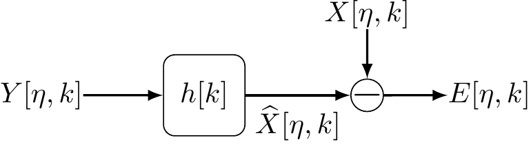
Consider estimating a desired signal X[k] from observations Y[k] using a linear filter with impulse response h[\kappa], producing the estimate \hat{X}[k] = \sum_{\kappa} h[\kappa] \, Y[k-\kappa]. The estimation error is E[k] = X[k] - \hat{X}[k].
- The optimal linear filter minimizes the mean squared error \mathbb{E}[E^2[k]] where E[k] = X[k] - \hat{X}[k]
- The orthogonality principle states that \mathbb{E}[E_{\min}[k] \cdot Y[k-\kappa]] = 0 for all \kappa
- The minimum estimation error E_{\min}[k] is orthogonal to all observations used in forming the estimate
- The optimal filter always achieves zero estimation error
- Orthogonality means the error is uncorrelated with the desired signal X[k]
- ✓ Correct. The MSE criterion \mathbb{E}[(X[k] - \hat{X}[k])^2] is the standard optimality criterion for linear estimation.
- ✓ Correct. The minimum-error signal is orthogonal to (uncorrelated with) all observations used in the estimate. This is the necessary and sufficient condition for optimality.
- ✓ Correct. This is the geometric interpretation: the optimal estimate is the projection of X[k] onto the subspace spanned by the observations, and the error is perpendicular to that subspace.
- ✗ Incorrect. Zero error would require X[k] to lie entirely in the subspace spanned by the observations, which is generally not the case. The MSE is minimized but typically remains nonzero.
- ✗ Incorrect. The orthogonality principle states that the error is uncorrelated with the observations Y[k-\kappa], not with the desired signal X[k]. These are different conditions.
Correct: The orthogonality principle is the cornerstone of linear optimal filtering: the estimation error must be orthogonal to every observation used. Geometrically, the optimal estimate is the orthogonal projection of the desired signal onto the observation subspace.
Review: Review the orthogonality condition carefully: \mathbb{E}[E_{\min}[k] \cdot Y[k-\kappa]] = 0 involves the observations Y, not the desired signal X. Also note that minimum MSE does not mean zero MSE.
Q091 Wiener–Hopf Equation
The equation determining the optimal linear filter
Which of the following statements about the Wiener–Hopf equation are correct?
The optimal linear filter h_{\text{opt}}[\kappa] satisfies the Wiener–Hopf equation, relating the cross-correlation R_{XY}[\kappa] and the autocorrelation R_{YY}[\kappa] of the involved processes.
- The Wiener–Hopf equation in the time domain is R_{XY}[\kappa] = \sum_{\lambda} h_{\text{opt}}[\lambda] \, R_{YY}[\kappa - \lambda], i.e., a convolution
- In the frequency domain, the optimal filter transfer function is H_{\text{opt}}(e^{j\Omega}) = S_{XY}(e^{j\Omega}) / S_{YY}(e^{j\Omega})
- The optimal filter is H_{\text{opt}}(e^{j\Omega}) = S_{XX}(e^{j\Omega}) / S_{YY}(e^{j\Omega})
- The optimal filter is H_{\text{opt}}(e^{j\Omega}) = S_{XY}(e^{j\Omega}) \cdot S_{YY}(e^{j\Omega})
- The Wiener–Hopf equation can only be solved in the time domain
- ✓ Correct. This convolution equation follows directly from applying the orthogonality principle and expresses the optimal filter in terms of the second-order statistics of the signals.
- ✓ Correct. Taking the DTFT of the Wiener–Hopf equation converts the convolution to a division of the cross-power spectral density by the auto-power spectral density of the observation.
- ✗ Incorrect. The numerator must be the cross-spectral density S_{XY}, not the auto-spectral density S_{XX}. The filter relates the desired output to the observation, requiring their cross-spectrum.
- ✗ Incorrect. The Wiener–Hopf equation in the frequency domain involves division by S_{YY}, not multiplication. Multiplication would amplify rather than equalize the observation spectrum.
- ✗ Incorrect. The frequency-domain formulation H_{\text{opt}} = S_{XY}/S_{YY} is often simpler and more insightful, especially for non-causal filters.
Correct: The Wiener–Hopf equation links the optimal filter to the second-order statistics (correlations and spectra) of the desired and observed signals. In the frequency domain, it becomes a simple ratio: cross-spectrum over observation auto-spectrum.
Review: Review the derivation: apply the orthogonality principle, then transform to the frequency domain. The key formula is H_{\text{opt}} = S_{XY}/S_{YY}, not S_{XX}/S_{YY} or S_{XY} \cdot S_{YY}.
§ 5.3 Wiener Filter
Q092 Wiener Filter
Optimal filtering for signal extraction from noisy observations
Which of the following statements about the Wiener filter are correct?
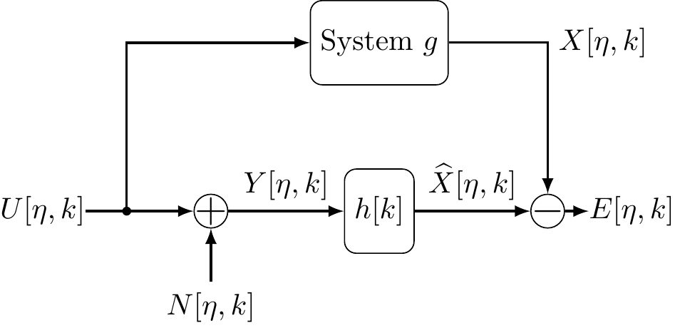
In the standard model, the observation is Y[k] = U[k] + N[k] (signal plus noise), and the desired output is X[k] = (g * U)[k] where g[\kappa] is a known system. U and N are assumed orthogonal (uncorrelated).
- In the standard model Y = U + N with desired output X = g * U, the optimal filter is H_{\text{opt}}(e^{j\Omega}) = G(e^{j\Omega}) \cdot \frac{S_{UU}(e^{j\Omega})}{S_{UU}(e^{j\Omega}) + S_{NN}(e^{j\Omega})}
- When S_{NN} \to 0 (no noise), H_{\text{opt}} \to G; when S_{NN} \to \infty (pure noise), H_{\text{opt}} \to 0
- The Wiener filter trades off signal fidelity against noise suppression based on the frequency-dependent SNR
- The Wiener filter amplifies noise at frequencies where the signal is weak
- The optimal filter is H_{\text{opt}} = G regardless of the signal-to-noise ratio
- ✓ Correct. This decomposes into the desired system G multiplied by a noise-suppression factor S_{UU}/(S_{UU}+S_{NN}) that depends on the signal-to-noise ratio at each frequency.
- ✓ Correct. With no noise, the filter applies G perfectly. With overwhelming noise, the filter suppresses everything to avoid amplifying noise.
- ✓ Correct. At frequencies where S_{UU} \gg S_{NN}, the filter passes the signal; where S_{NN} \gg S_{UU}, it attenuates. This is the fundamental SNR-dependent behavior.
- ✗ Incorrect. The Wiener filter attenuates at frequencies where the signal is weak relative to noise (S_{NN} \gg S_{UU}), because S_{UU}/(S_{UU}+S_{NN}) \to 0 in that regime.
- ✗ Incorrect. H_{\text{opt}} = G only when there is no noise (S_{NN} = 0). In general, the noise-suppression factor S_{UU}/(S_{UU}+S_{NN}) modifies G to balance fidelity and noise rejection.
Correct: The Wiener filter optimally balances two objectives: applying the desired system G to the signal, and suppressing noise. The key factor S_{UU}/(S_{UU}+S_{NN}) acts as a frequency-dependent weight controlled by the local SNR.
Review: Review the Wiener filter formula and its limiting cases. The filter does not simply apply G — it also accounts for noise. At low-SNR frequencies, it attenuates rather than amplifies.
Q093 Smoothing, Filtering, and Prediction
Distinguishing the three modes of optimal linear estimation
Which of the following statements about smoothing, filtering, and prediction are correct?
In the optimal filter framework, the desired output X[k] may represent a time-shifted version of the useful signal: X[k] = U[k - k_0]. The value of k_0 determines the estimation mode.
- Smoothing (k_0 > 0) estimates a past signal value and is generally easier (lower MSE) than filtering, because it effectively uses “future” observations
- Prediction (k_0 < 0) estimates a future signal value and typically has the highest MSE among the three modes
- Smoothing, filtering, and prediction are all realized by the same Wiener filter formula with different values of k_0 in the desired output definition
- Prediction is always more accurate than filtering because it extrapolates the signal trend
- Filtering and smoothing are identical operations
- ✓ Correct. With k_0 > 0, we estimate U[k-k_0] (a past value) from Y[k] (current observation), which includes information about the future relative to the target time. This extra information reduces the MSE.
- ✓ Correct. Predicting ahead is inherently harder because no future information is available. The farther ahead we predict, the larger the MSE.
- ✗ Incorrect. While all three use the Wiener framework, they are different problems with different optimal filter solutions. The value of k_0 changes the cross-spectral density S_{XY}, leading to a different H_{\text{opt}} for each mode.
- ✗ Incorrect. Prediction is generally less accurate than filtering. Estimating future values from current/past data introduces additional uncertainty compared to estimating the current value.
- ✗ Incorrect. Filtering (k_0 = 0) estimates the current signal value, while smoothing (k_0 > 0) estimates a past value using additional future information. They have different optimal filters and different MSEs.
Correct: The parameter k_0 determines the estimation task: smoothing (k_0 > 0, past), filtering (k_0 = 0, present), prediction (k_0 < 0, future). MSE generally increases from smoothing to filtering to prediction, because less relevant information is available.
Review: Review the role of k_0: it shifts the target relative to the observation time. Smoothing benefits from “future” observations relative to the target, making it easier than filtering, which in turn is easier than prediction.
Q094 Causal FIR Wiener Filter
Matrix formulation of the optimal causal finite impulse response filter
Which of the following statements about the causal FIR Wiener filter are correct?
For a causal FIR filter of order P, \hat{X}[k] = \sum_{\kappa=0}^{P} h[\kappa] \, Y[k-\kappa], the optimal coefficients are found by solving a system of linear equations derived from the Wiener–Hopf equation.
- The causal FIR optimal filter coefficients satisfy the matrix equation \mathbf{R}_{YY} \cdot \mathbf{h}_{\text{opt}} = \mathbf{r}_{XY}, the Wiener–Hopf equation in matrix form
- For a WSS process, the autocorrelation matrix \mathbf{R}_{YY} has Toeplitz structure
- The causal FIR filter always achieves the same MSE as the non-causal (unrestricted) Wiener filter
- The Toeplitz structure of \mathbf{R}_{YY} requires the observation noise to be white
- The causal FIR filter always has lower MSE than the non-causal Wiener filter
- ✓ Correct. The orthogonality principle for finite causal filters yields this system, where \mathbf{R}_{YY} is the autocorrelation matrix of Y and \mathbf{r}_{XY} is the cross-correlation vector.
- ✓ Correct. Wide-sense stationarity means R_{YY}[m,n] depends only on |m-n|, giving the matrix constant diagonals (Toeplitz structure), which can be exploited for efficient computation (e.g., Levinson–Durbin algorithm).
- ✗ Incorrect. Restricting the filter to be causal and finite-order removes degrees of freedom, so the MSE is generally higher than for the unrestricted (non-causal, IIR) Wiener filter.
- ✗ Incorrect. The Toeplitz structure comes from wide-sense stationarity of Y[k], regardless of whether the noise is white or colored.
- ✗ Incorrect. The non-causal filter uses both past and future observations and has no order constraint, so it achieves equal or lower MSE. Restricting to causal FIR can only increase the MSE.
Correct: The causal FIR Wiener filter is the practical version of optimal filtering: the normal equations \mathbf{R}_{YY} \mathbf{h} = \mathbf{r}_{XY} form a Toeplitz system (for WSS processes) that can be solved efficiently. The price of causality and finite order is a higher MSE compared to the unconstrained Wiener filter.
Review: Review the matrix formulation and the source of the Toeplitz structure (stationarity, not white noise). Remember that restricting the filter class (causal, finite order) can only increase or maintain the MSE.
Q095 Linear Prediction
Predicting future signal values from past observations
Which of the following statements about linear prediction are correct?
A linear predictor of order P estimates X[k] from P past values: \hat{X}[k] = \sum_{i=1}^{P} a_i \, X[k-i] The optimal coefficients a_i minimize \mathbb{E}[(X[k] - \hat{X}[k])^2].
- Linear prediction estimates X[k] from past values X[k-1], X[k-2], \ldots, X[k-P]
- The optimal predictor coefficients satisfy the Yule–Walker equations, also known as LPC (linear predictive coding) equations
- For an AR(P) process, the prediction error of the optimal order-P predictor is white noise
- The optimal linear predictor always achieves zero prediction error
- The prediction order P has no effect on the quality of the prediction
- ✓ Correct. The predictor uses a weighted sum of the P most recent past values to estimate the current (or next) sample.
- ✓ Correct. Applying the orthogonality principle yields the Yule–Walker system \mathbf{R}_{XX} \mathbf{a} = \mathbf{r}_{XX}, which has the same Toeplitz structure as the Wiener–Hopf matrix equation.
- ✓ Correct. An AR(P) process is generated by filtering white noise, so the optimal order-P predictor exactly inverts this and the residual is the original white noise driving process.
- ✗ Incorrect. Zero error would require X[k] to be perfectly determined by its past, which is only true for deterministic signals. For stochastic processes, there is always a residual prediction error.
- ✗ Incorrect. Increasing P generally reduces the prediction error (or at least does not increase it), because a higher-order predictor can capture more of the signal’s temporal structure.
Correct: Linear prediction uses past samples to estimate the current value. The Yule–Walker (LPC) equations give the optimal coefficients. For AR processes of matching order, the prediction error equals the driving white noise. Higher prediction orders generally improve accuracy.
Review: Review the Yule–Walker equations and the connection to AR processes. The prediction order P matters — higher orders capture more structure. Perfect prediction is impossible for genuinely stochastic signals.
§ 5.4 Matched Filter
Q096 Matched Filter
Maximizing the output signal-to-noise ratio
Which of the following statements about the matched filter are correct?
The matched filter is designed to detect a known signal u[k] in additive noise. Unlike the Wiener filter, its optimality criterion is maximizing the output signal-to-noise ratio (SNR) at a specific sampling instant k_0.
- The matched filter maximizes the output SNR, not the MSE (unlike the Wiener filter)
- For white noise with PSD S_{NN} = \sigma_N^2, the optimal impulse response is h_{\text{opt}}[k] \propto u[k_0 - k], i.e., the time-reversed and shifted known signal
- The maximum output SNR depends on the signal energy E_u = \sum_k |u[k]|^2 divided by the noise variance
- The matched filter minimizes the mean squared error
- The matched filter impulse response is h_{\text{opt}}[k] = u[k] (no time reversal needed)
- ✓ Correct. The Wiener filter minimizes MSE, while the matched filter maximizes the peak SNR at the decision time. These are fundamentally different criteria.
- ✓ Correct. The matched filter is literally “matched” to the signal shape by correlating the observation with a time-reversed copy of the expected signal.
- ✓ Correct. The peak output SNR is \text{SNR}_{\max} = E_u / \sigma_N^2, depending only on the total signal energy and the noise level.
- ✗ Incorrect. MSE minimization is the Wiener filter criterion. The matched filter maximizes the output SNR at a specific time instant, which is a different optimization problem.
- ✗ Incorrect. Time reversal is essential: h_{\text{opt}}[k] \propto u[k_0 - k]. Without reversal, the filter computes convolution instead of correlation, and the SNR is not maximized.
Correct: The matched filter is the optimal detector for a known signal in noise: it correlates the input with the expected signal shape (time-reversed) to maximize the output SNR at the decision instant. The achievable SNR depends on the signal’s total energy relative to the noise power.
Review: Review the difference between Wiener (MSE) and matched filter (SNR) criteria. The time-reversal in the matched filter impulse response is crucial — it converts convolution into correlation.
Q097 Matched Filter for Colored Noise
Extending the matched filter to non-white noise environments
Which of the following statements about the matched filter in colored noise are correct?
When the noise N[k] has a non-flat power spectral density S_{NN}(e^{j\Omega}) (colored noise), the matched filter must account for the frequency-dependent noise power.
- For colored noise, the optimal filter in the frequency domain is H_{\text{opt}}(e^{j\Omega}) \propto \frac{U^*(e^{j\Omega}) \, e^{-j\Omega k_0}}{S_{NN}(e^{j\Omega})}
- The colored-noise matched filter effectively pre-whitens the noise before applying the standard matched filter
- The matched filter for colored noise is identical to the white-noise matched filter
- The noise PSD S_{NN}(e^{j\Omega}) does not appear in the optimal filter formula
- The maximum output SNR is independent of the noise color (spectral shape)
- ✓ Correct. The noise spectrum appears in the denominator, effectively de-emphasizing frequencies where the noise is strong. This generalizes the white-noise matched filter.
- ✓ Correct. Dividing by S_{NN}(e^{j\Omega}) normalizes the noise to unit spectral density, after which the standard (white-noise) matched filter structure applies.
- ✗ Incorrect. Colored noise requires accounting for the frequency-dependent noise power S_{NN}(e^{j\Omega}). Only when S_{NN} is constant (white noise) do the two filters coincide.
- ✗ Incorrect. S_{NN} appears in the denominator of H_{\text{opt}}, weighting frequencies inversely proportional to the noise power to achieve the maximum SNR.
- ✗ Incorrect. The achievable SNR depends on how the signal energy is distributed relative to the noise spectrum. Colored noise can improve or degrade the SNR compared to white noise with the same total power, depending on the spectral overlap.
Correct: The colored-noise matched filter generalizes the white-noise result by incorporating S_{NN}(e^{j\Omega}) in the denominator. This pre-whitening interpretation shows the two-step structure: first equalize the noise, then correlate with the signal.
Review: Review how the noise spectrum enters the matched filter formula. The key idea is pre-whitening: dividing by S_{NN} normalizes the noise, and then the standard matched filter structure applies. The achievable SNR depends on the spectral relationship between signal and noise.
Ch 6 — Hilbert Spaces
§ 6.1 Inner Product Spaces
Q098 Inner Product of Random Variables
The Hilbert space structure of square-integrable random variables
Which of the following statements about the inner product of random variables are correct?
The space L^2(\Omega) of square-integrable random variables can be equipped with an inner product, turning it into a Hilbert space. This provides a geometric framework for estimation.
- The inner product for random variables is defined as \langle X, Y \rangle = \mathbb{E}[X Y^*]
- For zero-mean random variables, orthogonality \langle X, Y \rangle = 0 is equivalent to being uncorrelated: \mathbb{E}[XY^*] = 0
- MMSE estimation corresponds to orthogonal projection in L^2(\Omega)
- The inner product of two random variables is \langle X, Y \rangle = \mathbb{E}[X + Y]
- Orthogonality of random variables implies statistical independence
- ✓ Correct. This defines a valid inner product on L^2(\Omega): it is linear, conjugate-symmetric, and positive definite (up to almost-sure equality).
- ✓ Correct. For zero-mean variables, \mathbb{E}[XY^*] = \text{Cov}(X,Y), so orthogonality and uncorrelatedness coincide.
- ✓ Correct. The optimal estimate is the projection of the target random variable onto the subspace spanned by the observations, and the error is orthogonal to that subspace — exactly the orthogonality principle.
- ✗ Incorrect. The inner product is \mathbb{E}[XY^*] (expectation of the product), not \mathbb{E}[X+Y] (expectation of the sum).
- ✗ Incorrect. Orthogonality (\mathbb{E}[XY^*] = 0) means uncorrelated (for zero-mean), which is weaker than independence. Independence implies uncorrelatedness, but not vice versa.
Correct: The inner product \langle X, Y \rangle = \mathbb{E}[XY^*] gives L^2(\Omega) a Hilbert space structure, where orthogonality corresponds to being uncorrelated (for zero-mean variables). MMSE estimation is simply orthogonal projection in this space.
Review: Review the definition of the inner product (\mathbb{E}[XY^*], not \mathbb{E}[X+Y]) and the distinction between orthogonality/uncorrelatedness and statistical independence. Uncorrelatedness is a second-order property; independence is much stronger.
§ 6.3 Projections and the Gramian
Q099 Gram Matrix and Normal Equations
The algebraic structure of optimal estimation in Hilbert space
Which of the following statements about the Gram matrix in the context of optimal estimation are correct?
Given observation random variables \{X_1, X_2, \ldots, X_P\} and a target Y, the optimal linear estimate \hat{Y} = \sum_i a_i X_i is determined by the normal equations involving the Gram matrix.
- The Gram matrix has entries G_{ij} = \langle X_i, X_j \rangle = \mathbb{E}[X_i X_j^*]
- The normal equations \mathbf{G} \cdot \mathbf{a} = \mathbf{b} where b_i = \langle Y, X_i \rangle have the same structure as the Wiener–Hopf equation
- The Gram matrix is always diagonal
- The Gram matrix is identical to the covariance matrix for any set of random variables
- The normal equations require that the observation variables form a linearly independent set
- ✓ Correct. The Gram matrix collects all pairwise inner products of the observation variables, capturing their correlation structure.
- ✓ Correct. The Wiener–Hopf equation \mathbf{R}_{YY}\mathbf{h} = \mathbf{r}_{XY} is the concrete realization of these abstract normal equations for WSS processes.
- ✗ Incorrect. The Gram matrix is diagonal only when all observation variables are mutually orthogonal (uncorrelated for zero-mean). In general, the off-diagonal entries are nonzero.
- ✗ Incorrect. The Gram matrix equals the covariance matrix only for zero-mean variables. In general, G_{ij} = \mathbb{E}[X_i X_j^*] includes the means, while \text{Cov}(X_i, X_j) = \mathbb{E}[(X_i - m_i)(X_j - m_j)^*].
- ✗ Incorrect. The normal equations can always be formulated; if the observations are linearly dependent, the Gram matrix is singular but the equations are still consistent (the solution may not be unique). The optimal estimate itself is unique regardless.
Correct: The Gram matrix \mathbf{G} encodes the inner products (correlations) of the observations, and the normal equations \mathbf{G}\mathbf{a} = \mathbf{b} determine the optimal coefficients. This abstract formulation unifies the Wiener–Hopf equation, Yule–Walker equations, and other linear estimation problems.
Review: Review the distinction between the Gram matrix (\mathbb{E}[X_i X_j^*]) and the covariance matrix (which subtracts means). The Gram matrix is not generally diagonal, and the normal equations do not strictly require linear independence of observations.
Q100 Projection in Hilbert Space
The geometric interpretation of optimal estimation
Which of the following statements about projection in Hilbert space for optimal estimation are correct?
In L^2(\Omega), estimating a random variable Y from observations \{X_1, \ldots, X_P\} is equivalent to projecting Y onto the subspace \mathcal{V} = \text{span}\{X_1, \ldots, X_P\}.
- Optimal linear estimation is the orthogonal projection of the target Y onto the subspace spanned by the observations
- The projection minimizes the distance (= MSE) between the target Y and its estimate \hat{Y}
- The Wiener filter is the concrete realization of this projection for WSS processes observed through a linear filter
- Projection in L^2(\Omega) can always achieve zero estimation error for any target
- The Hilbert space framework for estimation applies only to Gaussian random variables
- ✓ Correct. The estimate \hat{Y} \in \mathcal{V} is the unique element of \mathcal{V} closest to Y in the MSE sense, which is exactly the orthogonal projection.
- ✓ Correct. By the projection theorem, \|Y - \hat{Y}\|^2 = \mathbb{E}[|Y - \hat{Y}|^2] is minimized when \hat{Y} is the orthogonal projection of Y onto \mathcal{V}.
- ✓ Correct. The abstract Hilbert space projection becomes the Wiener–Hopf equation when the observations are samples of a WSS process. The Wiener filter coefficients implement the projection.
- ✗ Incorrect. Zero error requires Y \in \mathcal{V}, i.e., the target must be a linear combination of the observations. In general, Y has a component orthogonal to \mathcal{V} that cannot be recovered.
- ✗ Incorrect. The L^2(\Omega) framework applies to any square-integrable random variables, regardless of their distribution. It uses only second-order statistics (means, correlations), which exist for all L^2 variables.
Correct: The Hilbert space perspective unifies all linear estimation problems: MMSE estimation is orthogonal projection, the error is perpendicular to the observation subspace, and the Wiener filter is the concrete implementation for WSS processes. This framework is distribution-free — it requires only finite second moments.
Review: Review the projection theorem in Hilbert spaces: the projection minimizes the distance but generally cannot make it zero. The framework uses only inner products (second-order statistics) and applies to any distribution, not just Gaussian.