Chapter 4 — Introduction to Estimation Theory
Companion material for Chapter 4. Covers classical and Bayesian parameter estimation, MLE, MAP, MMSE, the Cramér–Rao bound, regression, and hypothesis testing.
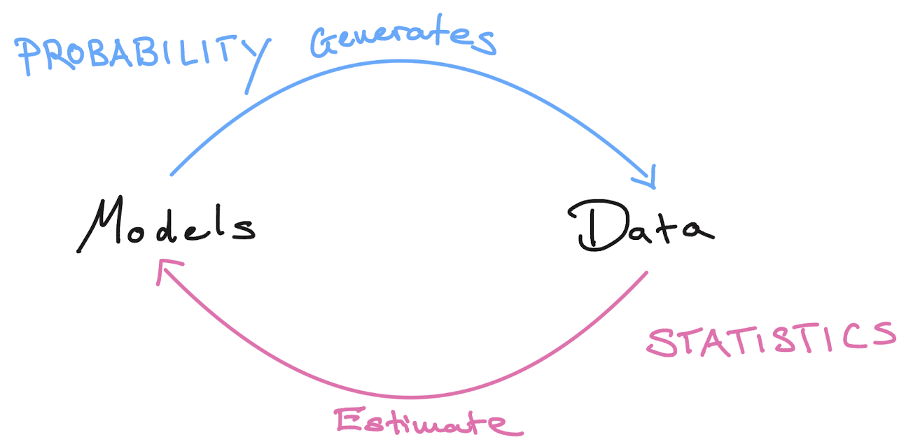
§ 4.1 Embedding in Statistics
Parameter Estimation Setup
Excursion: Plato’s Allegory of the Cave
§ 4.3 Parameter Estimation
Confidence Intervals
Build a confidence interval for the mean of an exponential random variable with the 68–95–99.7 rule, then resample to confirm that ~95% of the 95% intervals contain the true mean.
§ 4.4 Maximum Likelihood Estimation
MLE in Action
Maximum-likelihood classification on Fisher’s Iris data set, with class-conditional densities as likelihoods and ML decision regions for one and two features.
Excursion
🎥 Bayesian reasoning about coin flips — the MLE and MAP perspectives on the same estimation problem.
Estimate a Gaussian’s mean and variance from N measurements by sweeping a “hypothetical world” for each parameter and tracing the resulting likelihood.
§ 4.5 Bayesian Estimation
Did the sun explode?
Late one night a detector beeps: the Sun has exploded. Should you believe it? Reasoning about a hidden cause from an observation is exactly the job of Bayesian inference. Define two binary events:
- E — the Sun has exploded (complement \lnot E: it is intact);
- V — the Sun is visible in the sky (complement \lnot V: it is not).
What links the hidden state of the world E to the thing we can actually observe, V, is the likelihood — the conditional probability \mathbb{P}(V \mid E). Laid out over the two states of the world (columns) and the two possible observations (rows), it forms a 2\times 2 table. Each column sums to 1: fixing the state of the world, the Sun is either visible or not.
| E: Sun exploded | \lnot E: Sun intact | |
|---|---|---|
| V: Sun visible | \mathbb{P}(V \mid E) | \mathbb{P}(V \mid \lnot E) |
| \lnot V: not visible | \mathbb{P}(\lnot V \mid E) | \mathbb{P}(\lnot V \mid \lnot E) |
The table only runs cause \to observation. To answer the question we actually care about — given what I see, did the Sun explode? — we must run it backwards with Bayes’ theorem, which reweights the likelihood by the prior \mathbb{P}(E): \mathbb{P}(E \mid V) = \frac{\mathbb{P}(V \mid E)\,\mathbb{P}(E)}{\mathbb{P}(V)}. A spontaneous solar explosion is astronomically improbable, so the prior \mathbb{P}(E) is minuscule. Even a frightening observation — the Sun nowhere to be seen — is explained far more plausibly by a passing cloud or simple nightfall than by the end of the world. The likelihood table alone never settles it; the prior does. (After xkcd 1132, “Frequentists vs. Bayesians”.)
Choosing priors
What effect do the following priors have on the estimation?
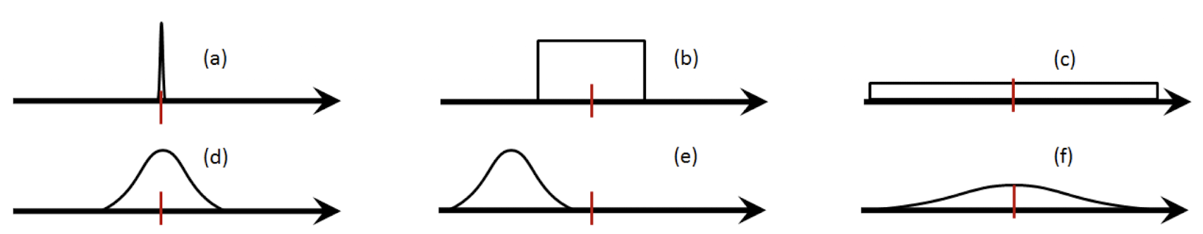
Which prior should we choose?
- Based on your preference, e.g., you know from historical data that the parameter should behave in certain ways.
- Based on physics, e.g., the parameter has a physical interpretation, so you need to abide by the physical laws.
- Choose a prior that is computationally “friendlier”. This is the topic of the conjugate prior, which is a prior that does not change the form of the posterior distribution.
Prior to Posterior
Sample random locations on Earth one by one and watch a uniform prior over the water fraction p sharpen into a posterior as observations accumulate.
MAP Estimator
Three steps on fusing two pieces of information about one unknown: (1) independent sources combine by multiplying their likelihoods (2) two unbiased Gaussians with different variances give the precision-weighted mean (3) MAP with a Gaussian prior and likelihood recovers the same formula with the prior as a “second measurement”
Bayesian Risk
A forager decides “eat” or “discard” under asymmetric costs, building the Bayes-risk rule from the posterior and cost matrix and rewriting it as a likelihood-ratio test.
§ 4.6 Cramér–Rao Bound
Fisher Information
Estimate a Bernoulli success probability \phi with the relative-frequency estimator and watch it meet the Cramér–Rao bound \phi(1-\phi)/N set by the Fisher information.
§ 4.7 Regression Estimation
The full slide deck for this section — predicting one random variable from another, the MMSE and linear-MMSE estimators, and the orthogonality principle.
Before specializing to the linear case, see the whole progression of estimation methods on one three-component Gaussian-mixture joint law f_{XY}(x,y).
Linear Regression
Cross-correlation based peak detection for estimating delay between two noisy observations — a concrete least-squares estimation example.
See least squares on N samples as a noisy estimate of the population MMSE line a_{\mathrm{MMSE}}=C_{XY}/\sigma_X^2 that converges as N\to\infty, with Tikhonov/ridge regularization taming ill-conditioned inputs.
The linear-MMSE story on real Iris data, where predicting one feature from two 96\%-correlated ones makes \mathbf R_{XX} ill-conditioned until ridge regularization stabilizes the coefficients.
§ 4.8 Hypothesis Testing
The full slide deck for this section — deciding between competing models from data: the likelihood-ratio test, Neyman–Pearson, and the ROC curve.
Binary Decision Problem and Likelihood Ratio Test
The Bayes-risk decision rule rewritten as a likelihood-ratio test, with the threshold set by the priors and asymmetric costs.
ROC Curve
Vary a threshold on an alarm score to trace the false-alarm/detection trade-off and mark the Neyman–Pearson operating point on the ROC curve.
Mean Tests
Repeated density measurements of a gold bar as a one-sample mean test, comparing the z-test (known \sigma_X) with the t-test (estimated \widehat\Sigma_X).