Hypothesis Testing
Deciding between competing models from data
Two hypotheses
\[
% Number sets
\newcommand{\Nat}{\mathbb{N}}
\newcommand{\Integer}{\mathbb{Z}}
\newcommand{\Real}{\mathbb{R}}
\newcommand{\Complex}{\mathbb{C}}
% Operators
\newcommand{\SNR}{\operatorname{SNR}}
\newcommand{\tr}{\operatorname{tr}}
\newcommand{\re}{\operatorname{Re}}
\newcommand{\im}{\operatorname{Im}}
\newcommand{\sign}{\operatorname{sign}}
\newcommand{\rect}{\operatorname{rect}}
\newcommand{\sinc}{\operatorname{si}}
\newcommand{\erf}{\operatorname{erf}}
\newcommand{\erfc}{\operatorname{erfc}}
\newcommand{\kurt}{\operatorname{kurt}}
\newcommand{\diag}{\operatorname{diag}}
\newcommand{\MSE}{\operatorname{MSE}}
\newcommand{\argmin}{\operatorname*{argmin}}
\newcommand{\argmax}{\operatorname*{argmax}}
\newcommand{\bias}{\operatorname{bias}}
\newcommand{\Bin}{\operatorname{Bin}}
% Delimiters
\newcommand{\paren}[1]{\left(#1\right)}
\newcommand{\bracket}[1]{\left[#1\right]}
\newcommand{\set}[1]{\left\{#1\right\}}
\newcommand{\abs}[1]{\left\lvert #1 \right\rvert}
\newcommand{\norm}[1]{\left\lVert #1 \right\rVert}
\newcommand{\ip}[1]{\left\langle #1 \right\rangle}
% Notation
\newcommand{\dd}{\,\mathrm{d}}
\newcommand{\tran}{^{\top}}
\newcommand{\conv}{\ast}
\newcommand{\conj}{^{*}}
\newcommand{\herm}{^{\mathsf{H}}}
\newcommand{\opt}{_{\star}}
% Expectation and variance
% \newcommand{\E}[1]{\mathbb{E}\!\left[#1\right]}
\newcommand{\E}[2][]{\mathbb{E}_{#1}\!\left[#2\right]}
\newcommand{\Var}[1]{\mathbb{V}\!\left[#1\right]}
% Distributions
\newcommand{\Gauss}{\mathcal{N}}
\newcommand{\Uniform}{\mathcal{U}}
\newcommand{\FT}{\mathcal{F}}
% Probability
\newcommand{\Prob}[1]{\mathbb{P}\!\left(#1\right)}
% Misc
\newcommand{\bsy}[1]{\boldsymbol{#1}}
\newcommand{\calR}{\mathcal{R}}
\newcommand{\calC}{\mathcal{C}}
\]
\[
H_0 \;\text{(null)} \qquad\text{vs.}\qquad H_1 \;\text{(alternative)}
\]
Two competing statistical models for the observation \(\mathbf{X}\).
A decision rule maps observations to a decision:
\[
\delta : \mathcal{X} \to \{0, 1\}, \qquad \widehat{H} = \delta(\mathbf{X})
\]
It partitions the observation space into decision regions:
\[
\mathcal{X}_1 = \{\mathbf{x} : \delta(\mathbf{x}) = 1\}, \qquad
\mathcal{X}_0 = \{\mathbf{x} : \delta(\mathbf{x}) = 0\}
\]
Errors and Probabilities
| \(H_0\) true |
correct silence \(P_S\) |
false alarm \(P_F\) |
| \(H_1\) true |
miss \(P_M\) |
detection \(P_D\) |
\[
P_F = \Prob{\widehat{H}=H_1 \mid H_0}, \quad
P_D = \Prob{\widehat{H}=H_1 \mid H_1}, \\
P_M = 1 - P_D, \quad P_S = 1 - P_F
\]
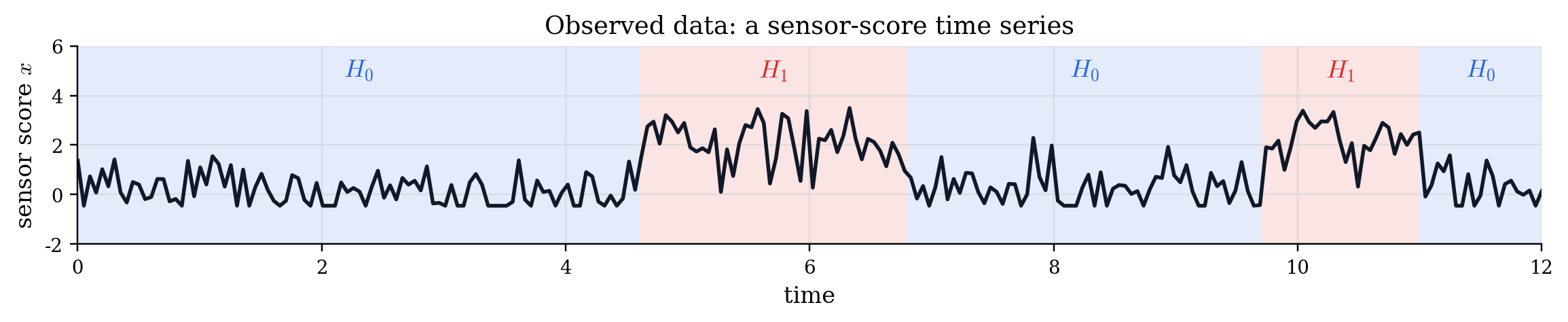
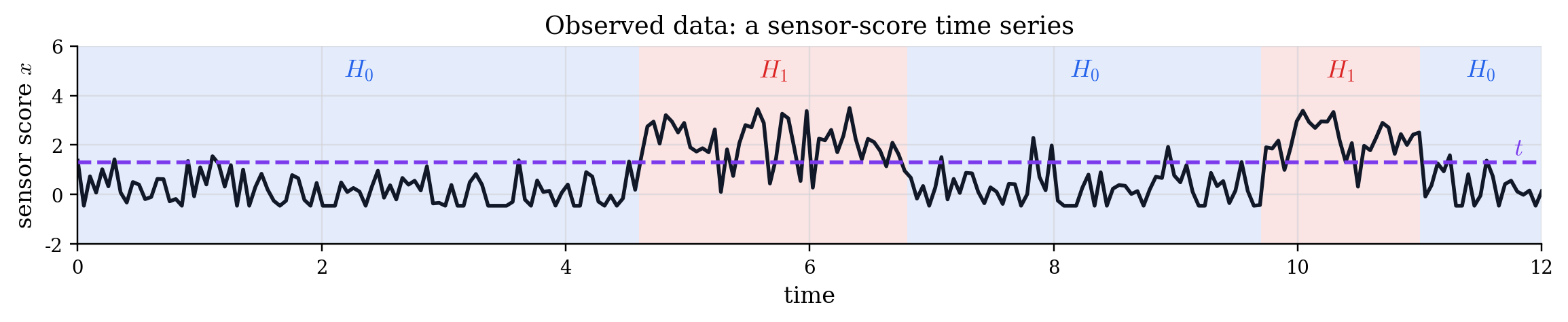
From data to ROC - Intruder Alarm
Sweeping the threshold
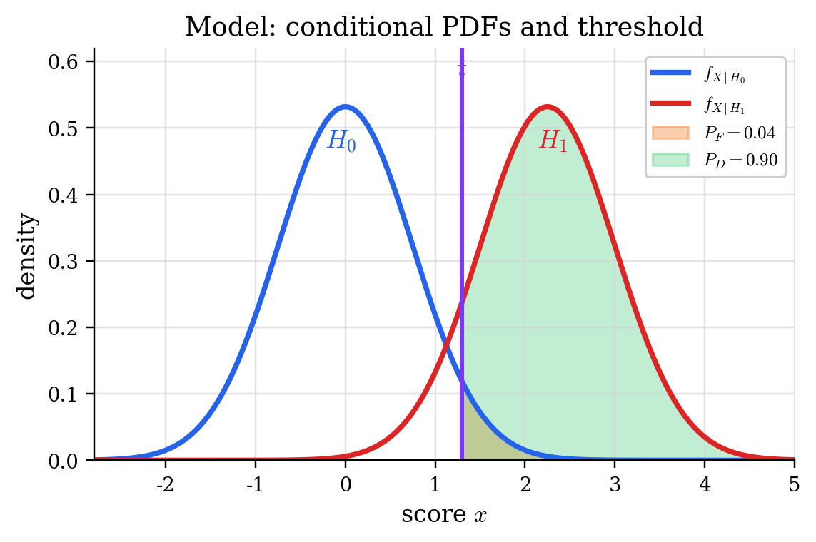
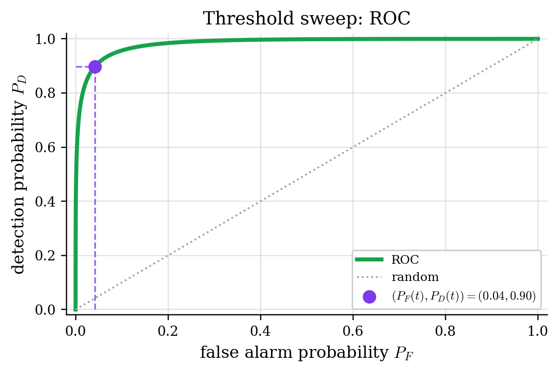
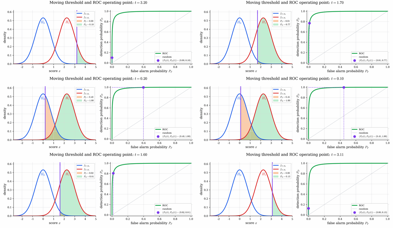
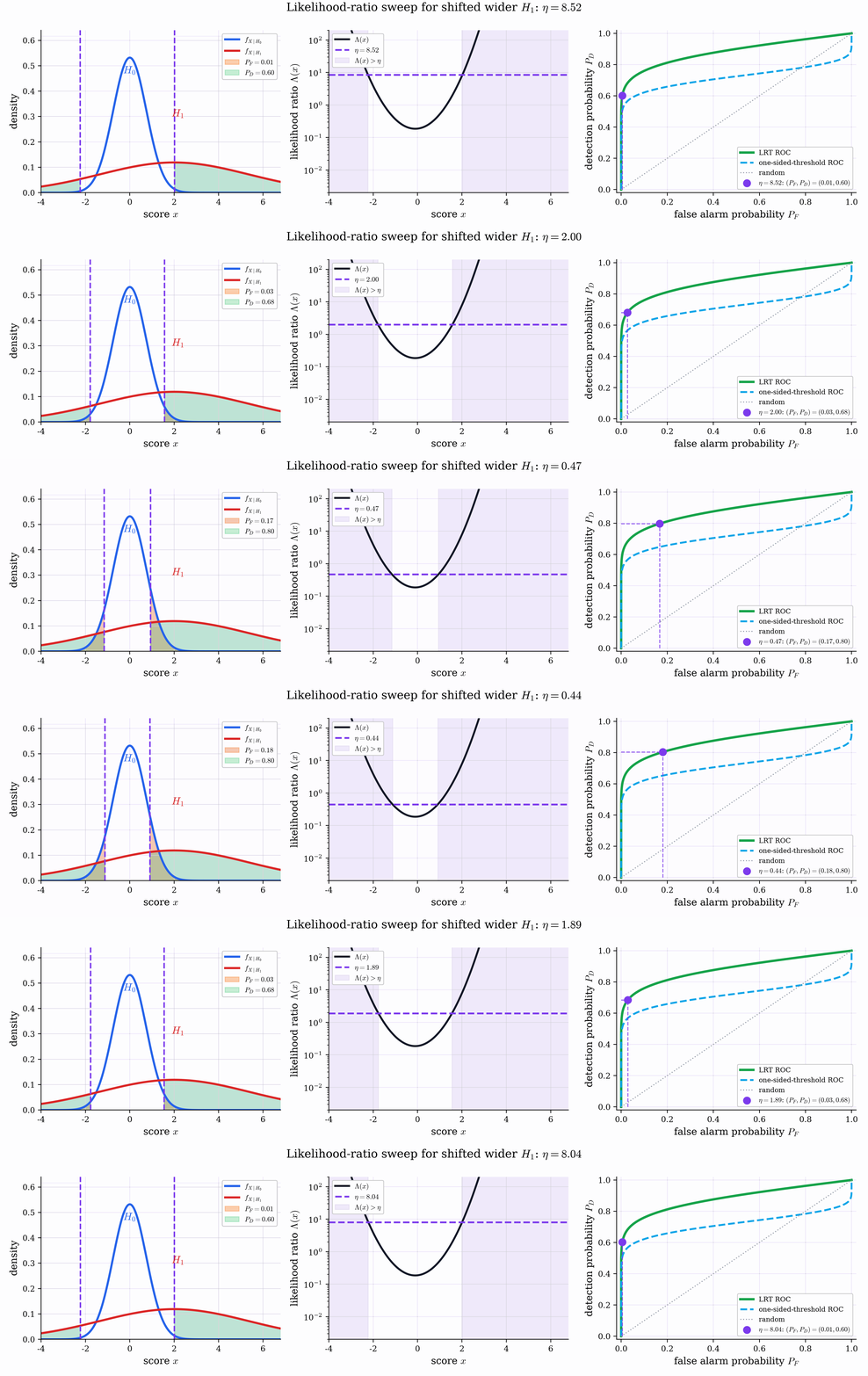
Sweeping the threshold \(t\) traces the Receiver Operating Characteristic (ROC) curve — \(P_D\) versus \(P_F\).
![]()
Fewer false alarms cost detections.
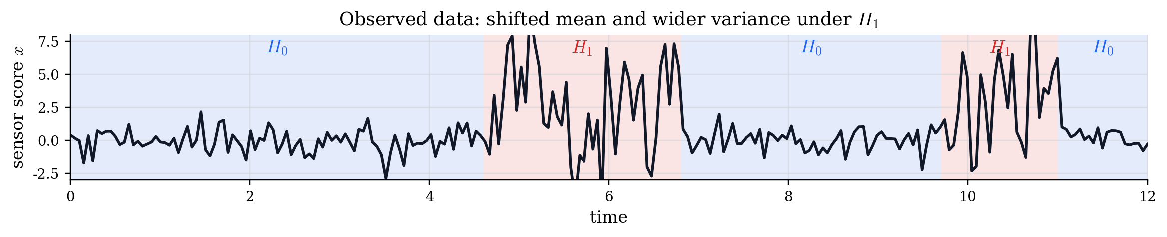
Another intruder alarm: wider variance
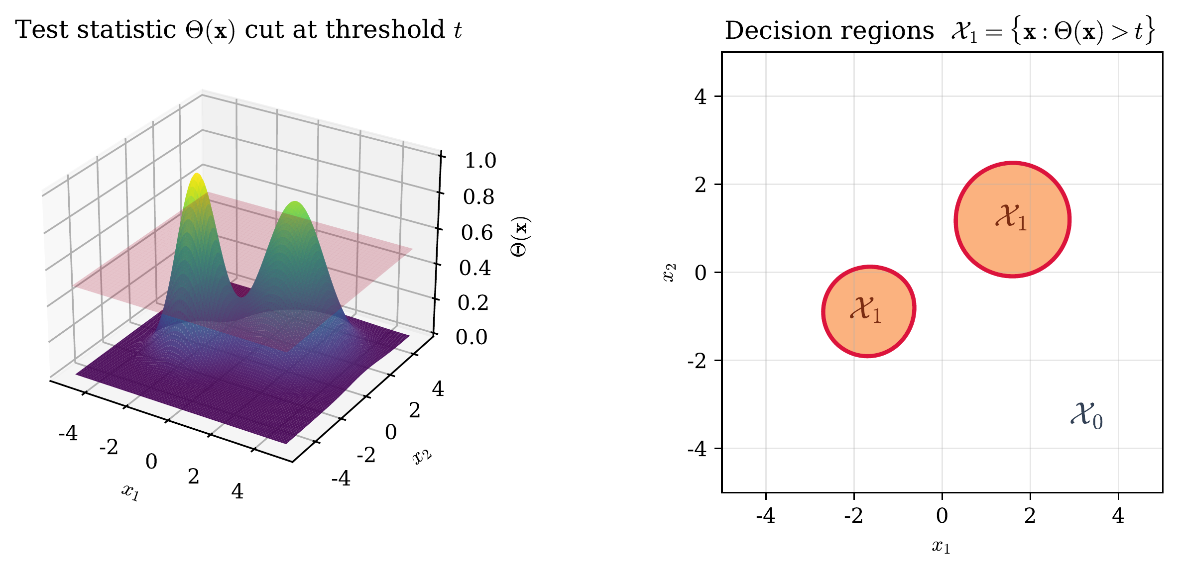
From a test statistic to regions
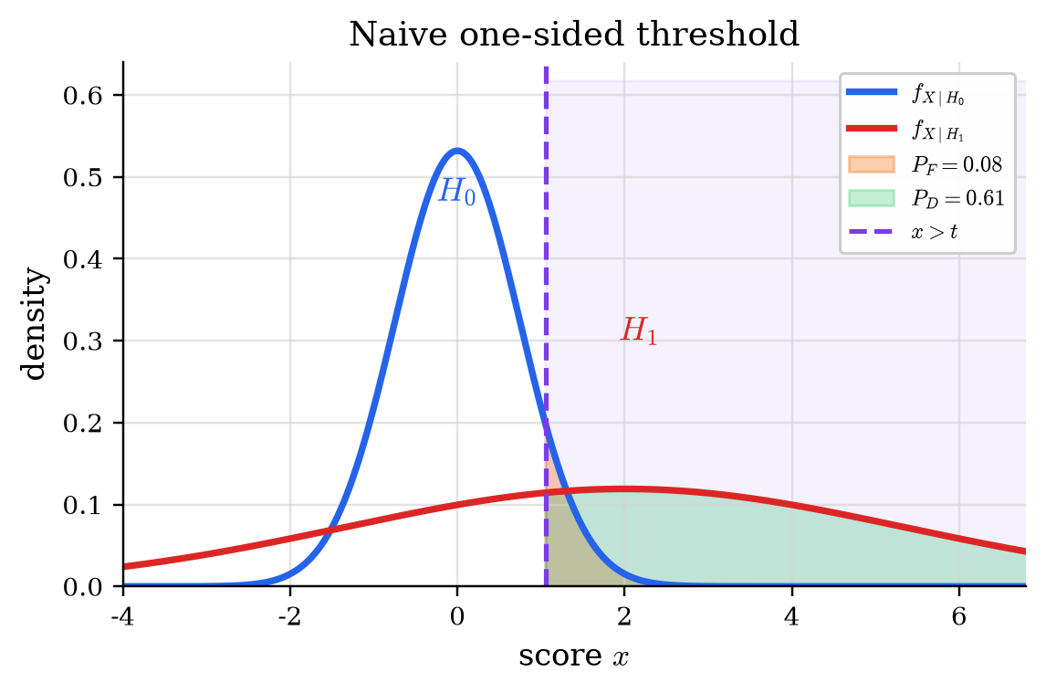
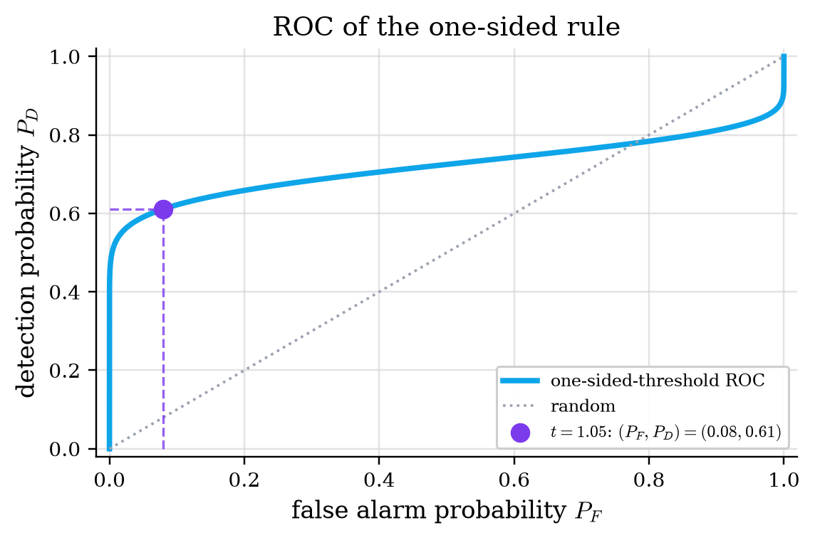
One common family of rules: threshold a test statistic \(\Theta(\mathbf{x})\).
\[
\Theta(\mathbf{x}) \underset{H_0}{\overset{H_1}{\gtrless}} t
\qquad\Longrightarrow\qquad
\mathcal{X}_1 = \{\mathbf{x} : \Theta(\mathbf{x}) > t\}
\]
![]()
Neyman–Pearson
When priors and costs are unknown, control the false-alarm rate:
Neyman–Pearson criterion Among all rules with \(P_F \le \alpha\), choose the one that maximizes \(P_D\).
Neyman–Pearson Lemma The optimal decision rule is a likelihood-ratio test:
\[
\Lambda(\mathbf{x}) = \frac{f_{\mathbf{X}\mid H_1}(\mathbf{x})}{f_{\mathbf{X}\mid H_0}(\mathbf{x})}
\;\underset{H_0}{\overset{H_1}{\gtrless}}\; \eta_\alpha,
\qquad \eta_\alpha \text{ chosen so that } P_F = \alpha
\]
This lemma requires simple hypotheses — no unknown parameters in \(f_{\mathbf{X}\mid H_i}\).
Non-simple hypotheses — Detecting counterfeit gold
Pure gold has density \(m_\text{gold} = 19.30\,\mathrm{g/cm^3}\). Measure \(N\) times, \(X_i \sim \Gauss(m, \sigma^2)\):
\[
H_0 : m = m_\text{gold} \quad\text{vs.}\quad H_1 : m \neq m_\text{gold}
\]
Under \(H_0\), the sample mean is Gaussian:
\[
\widehat{M} = \frac{1}{N}\sum_{i=1}^N X_i \;\sim\; \Gauss\!\left(m_\text{gold},\ \frac{\sigma^2}{N}\right)
\]
Reject \(H_0\) when \(\widehat{M}\) lands too far from \(m_\text{gold}\).
At \(\alpha = 5\%\): reject if more than 2 standard deviations away:
\[\;\bigl|\widehat{M} - m_\text{gold}\bigr| > 2\,\dfrac{\sigma}{\sqrt{N}}\;\]
Standardize: the z-test
Standardize the deviation into a single test statistic:
\[
Q = \frac{\widehat{M} - m_\text{gold}}{\sigma / \sqrt{N}}
\;\overset{H_0}{\sim}\; \Gauss(0, 1)
\]
The same rule becomes simply
\[
\boxed{\;\text{reject } H_0 \ \text{ if } \ |Q| > z_{1-\alpha/2}\;}
\qquad z_{0.975} \approx 2
\]
Known variance \(\sigma^2\) → z-test.
→ Demo: Gold Density Screening
Unknown variance: the t-test
In practice \(\sigma^2\) is unknown — estimate it from the same data:
\[
\widehat{\Sigma}^2 = \frac{1}{N-1}\sum_{i=1}^N (X_i - \widehat{M})^2
\]
\[
Q = \frac{\widehat{M} - m_\text{gold}}{\widehat{\Sigma} / \sqrt{N}}
\;\overset{H_0}{\sim}\; t_{N-1}
\quad\text{(Student-}t,\ N-1 \text{ d.o.f.)}
\]
How to choose an operating point
The likelihood-ratio test fixes the form of the optimal rule —
\[
\Lambda(\mathbf{x}) = \frac{f_{\mathbf{X}\mid H_1}(\mathbf{x})}{f_{\mathbf{X}\mid H_0}(\mathbf{x})}
\;\underset{H_0}{\overset{H_1}{\gtrless}}\; \eta
\]
— but which threshold \(\eta\)? Which point on the ROC?
Option 1 — fix the false-alarm rate. The Neyman–Pearson criterion:
\[
\eta = \eta_\alpha \quad\text{chosen so that}\quad P_F = \alpha
\]
Option 2 — minimize the Bayes risk. Set \(\eta\) from the costs \(C_{ij}\) and the hypothesis priors \(\Prob{H_i}\):
\[
\eta = \eta_{\text{Bayes}}
\]
Minimizing Bayes risk
If priors \(\Prob{H_i}\) and costs \(C_{ij} = \calC(\widehat{H}=H_i \mid H_j)\) are known, minimize the risk = expected cost:
\[
\calR(\delta) = \E{\calC(\widehat{H}, H)}
= \sum_{i,j} C_{ij}\, \Prob{\widehat{H}=H_i \mid H_j} \Prob{H_j}
\]
Leads to the Bayes risk test:
\[
\boxed{\;
\underbrace{\frac{f_{\mathbf{X}\mid H_1}(\mathbf{x})}{f_{\mathbf{X}\mid H_0}(\mathbf{x})}}_{\Lambda(\mathbf{x})}
\;\underset{H_0}{\overset{H_1}{\gtrless}}\;
\frac{\Prob{H_0}\,(C_{10}-C_{00})}{\Prob{H_1}\,(C_{01}-C_{11})} = \eta_{\text{Bayes}}
\;}
\]
Again a likelihood-ratio test — same form as Neyman–Pearson, different threshold.
Conditional risk
The Bayes risk can be written as an average over observations:
\[
\mathcal R(\delta)
= \int
\underbrace{
\mathcal R(\delta(\mathbf x) \mid \mathbf X=\mathbf x)}
_{\text{conditional risk}}
f_{\mathbf X}(\mathbf x)\,d\mathbf x .
\]
\[
\mathcal R(\delta(\mathbf x) \mid \mathbf X=\mathbf x) =
\E{\mathcal C(\delta(\mathbf x),H)\mid \mathbf X=\mathbf x}
\]
Hence, minimizing the total risk means choosing, for each observation \(\mathbf{x}\), the decision with smaller conditional risk.
For a fixed \(\mathbf{x}\), weigh the cost of each decision (conditional risk):
\[
\mathcal R(\delta(\mathbf x) = H_i \mid \mathbf X=\mathbf x) = \sum_{j} C_{ij}\, \Prob{H_j\mid \mathbf X=\mathbf x}
\]
Deriving the Posterior Odds Test
We compare the two conditional risks: \[
\calR(\delta(\mathbf x) = H_1 \mid \mathbf{x}) = C_{10}\,\Prob{H_0\mid\mathbf{x}} + C_{11}\,\Prob{H_1\mid\mathbf{x}}
\] \[
\calR(\delta(\mathbf x) = H_0 \mid \mathbf{x}) = C_{00}\,\Prob{H_0\mid\mathbf{x}} + C_{01}\,\Prob{H_1\mid\mathbf{x}}
\]
Decide \(H_1\) when it is the cheaper option,
\[\calR(\delta(\mathbf x) = H_0 \mid \mathbf{x}) > \calR(\delta(\mathbf x) = H_1 \mid \mathbf{x})\]
\[
(C_{01}-C_{11})\,\Prob{H_1\mid\mathbf{x}} \;>\; (C_{10}-C_{00})\,\Prob{H_0\mid\mathbf{x}}
\]
Thus, the decision rule is a posterior odds test: \[
\frac{\Prob{H_1\mid\mathbf{x}}}{\Prob{H_0\mid\mathbf{x}}}
\;\underset{H_0}{\overset{H_1}{\gtrless}}\;
\frac{(C_{10}-C_{00})}{(C_{01}-C_{11})}
\]
Deriving the likelihood-ratio test
Insert the posteriors \(\Prob{H_j\mid\mathbf{x}} = f_{\mathbf{X}\mid H_j}(\mathbf{x})\,\Prob{H_j} / f_{\mathbf{X}}(\mathbf{x})\) — the common \(f_{\mathbf{X}}(\mathbf{x})\) cancels:
\[
\Lambda(\mathbf{x}) = \frac{f_{\mathbf{X}\mid H_1}(\mathbf{x})}{f_{\mathbf{X}\mid H_0}(\mathbf{x})}
\;\underset{H_0}{\overset{H_1}{\gtrless}}\;
\frac{\Prob{H_0}\,(C_{10}-C_{00})}{\Prob{H_1}\,(C_{01}-C_{11})}
\]
Bayes’ rule recasts the test as an update of prior odds to posterior odds:
\[
\frac{\Prob{H_1 \mid \mathbf{x}}}{\Prob{H_0 \mid \mathbf{x}}}
= \Lambda(\mathbf{x}) \cdot \frac{\Prob{H_1}}{\Prob{H_0}}
\]