5 Architectural Acoustics
Lab Handbook - Assignment 4
This handbook provides the theoretical foundation for understanding architectural acoustics, focusing on early reflections modeling using the image method and wave domain modeling for room modes. These techniques are essential for simulating realistic acoustic environments in virtual acoustics.
5.1 Table of Contents
5.2 Introduction to Architectural Acoustics
5.2.1 From Free Field to Enclosed Spaces
In Assignment 1, we focused on free-field propagation, where sound travels directly from source to listener without any reflections. However, most real-world acoustic environments are enclosed spaces—rooms, halls, studios, and auditoria—where sound reflects off walls, floors, and ceilings.
Architectural acoustics deals with how sound behaves in enclosed spaces, including:
- Early reflections: Discrete echoes that arrive shortly after the direct sound
- Room modes: Resonant frequencies determined by room geometry
- Reverberation: Dense, diffuse sound field from many reflections
- Acoustic properties: How materials and geometry affect sound propagation
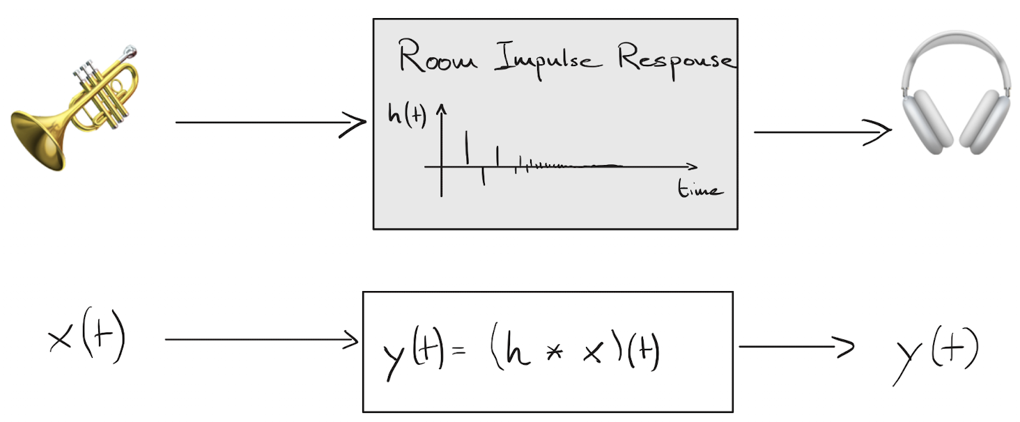
Auralization turns a room model into a listening experience: a real or simulated source is fed into a signal‑processing block that applies the room’s acoustic transfer function (typically the room impulse response) and outputs the sound as it would be heard at a listener position. In practice, this lets us compare designs, materials, or source/receiver positions by listening, not just measuring.
The video below shows a simulation of a wave in a concert hall, where the sound source is on the stage on the right.
5.2.2 The Complete Acoustic Response
In an enclosed space, the sound reaching a listener consists of:
- Direct sound: The sound that travels directly from source to listener (free-field component)
- Early reflections: Discrete echoes arriving within the first 50-100 ms after the direct sound
- Late reverberation: Dense, diffuse sound field from many overlapping reflections
The impulse response of a room captures all these components. It describes how a room responds to an impulsive sound source, containing information about:
- Arrival times of reflections
- Amplitudes and directions of reflections
- Frequency-dependent characteristics
- Reverberation decay
🎮 Application Spotlight: Project Acoustics
Project Acoustics brings advanced room acoustics modeling to game development and sound design. Leveraging the Triton technology from Microsoft Research, it provides realistic sound propagation based on wave physics—making virtual spaces sound as immersive as they look.
5.2.3 Assignment 4 Overview
This assignment introduces two fundamental techniques for modeling room acoustics:
Part 1: Early Reflections Modeling
- Using the image method to compute early reflections in a shoebox-shaped room
- Understanding how sound reflects off walls
- Implementing a simple yet effective model for small rooms
Part 2: Wave Domain Modeling
- Modeling low-frequency room modes using wave domain techniques
- Understanding how room geometry determines resonant frequencies
- Simulating the frequency response of a room with rigid boundaries
Together, these techniques provide a foundation for understanding how architectural spaces affect sound.
5.3 Early Reflections and the Image Method
5.3.1 What are Early Reflections?
Early reflections are discrete echoes that arrive at the listener shortly after the direct sound (typically within the first 50-100 milliseconds). Unlike late reverberation, which is diffuse and dense, early reflections are:
- Discrete: Each reflection can be identified as a separate event
- Directional: Each reflection arrives from a specific direction
- Geometrically determined: Their paths can be computed using geometric acoustics
Early reflections are crucial for:
- Spatial perception: They provide cues about room size and shape
- Source localization: They help listeners determine source position
- Speech intelligibility: They can enhance or degrade clarity
- Aesthetic quality: They contribute to the “acoustic character” of a space
5.3.2 Geometric Acoustics
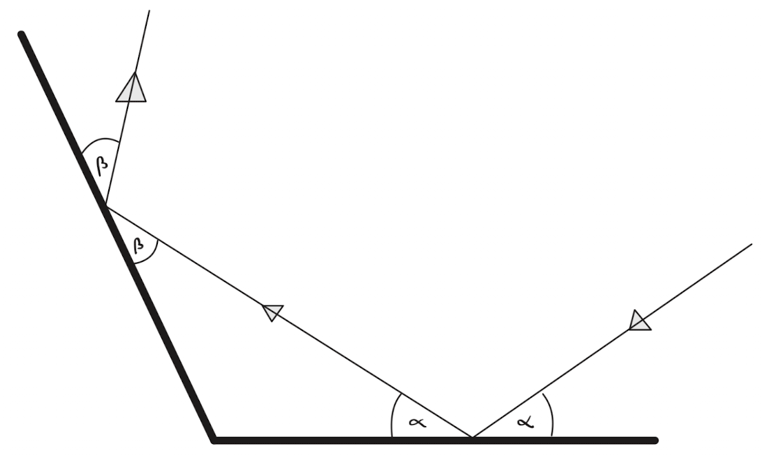
Geometric acoustics treats sound as rays that travel in straight lines and reflect off surfaces according to the law of reflection: the angle of incidence equals the angle of reflection. This approximation is valid when:
- The wavelength is much smaller than the room dimensions
- Surfaces are large compared to the wavelength
- We focus on high-frequency behavior (typically > 100-200 Hz)
For early reflections, geometric acoustics provides an efficient and accurate method for computing reflection paths. At InteractiveAcoustics.info, you can learn about the fundamentals of geometrical acoustics through interactive tutorials and examples.
5.3.3 The Image Source Method
The image source method (ISM) is an elegant technique for computing early reflections in rectangular rooms. It was introduced by Allen and Berkley (1979) and remains one of the most efficient methods for shoebox-shaped rooms.
5.3.3.1 Basic Concept
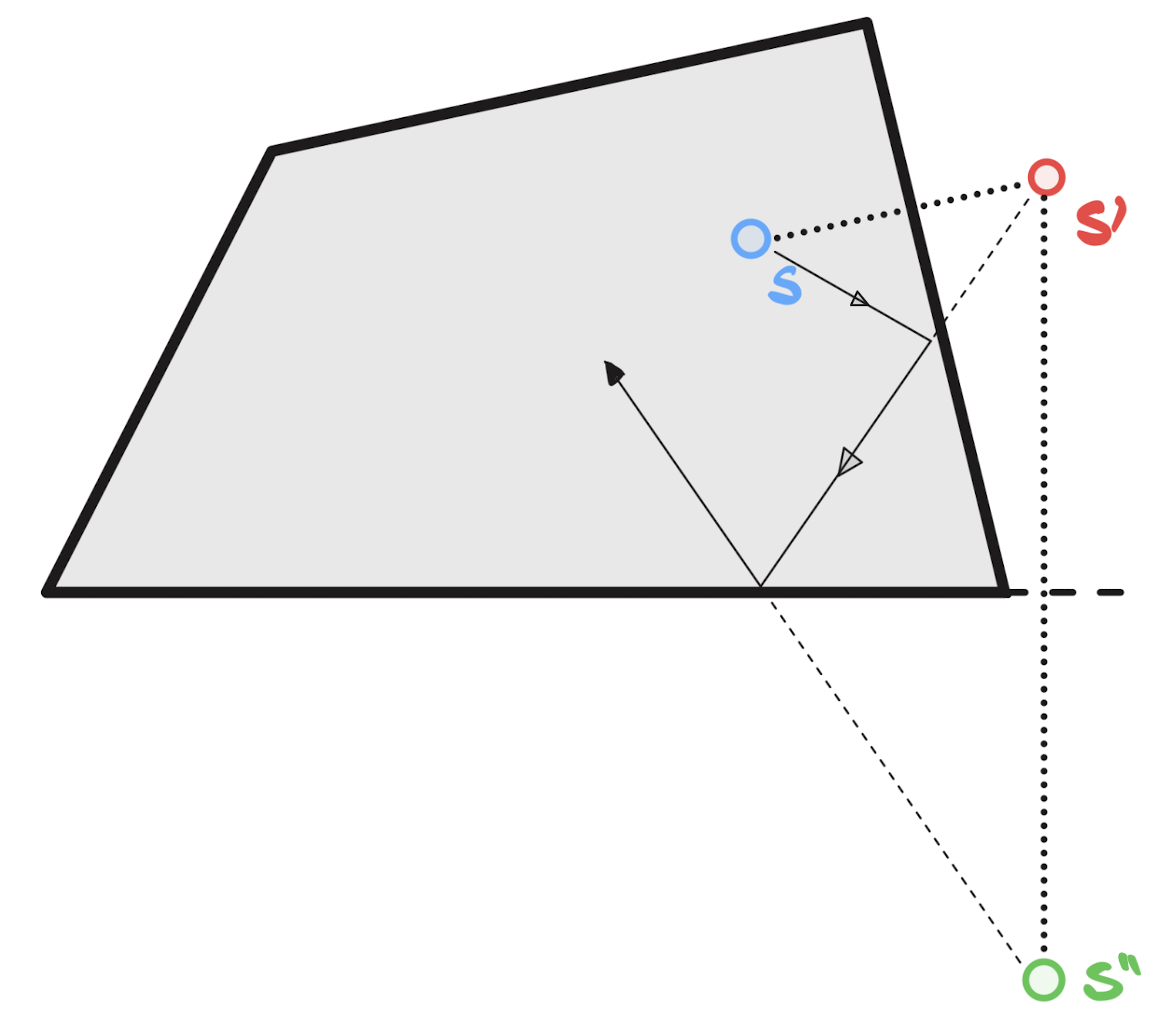
Instead of tracing rays as they reflect off walls, the image method creates virtual image sources by mirroring the real source across each wall. The path from an image source to the listener corresponds to a reflection path in the real room.
5.3.3.2 Single Reflection Example
Consider a 2D room with a source at position (x_s, y_s) and a listener at (x_l, y_l). To find the reflection off the right wall (at x = W):
Create an image source by mirroring the real source across the right wall: x_{img} = 2W - x_s, \quad y_{img} = y_s
Compute the path from the image source to the listener: d = \sqrt{(x_{img} - x_l)^2 + (y_{img} - y_l)^2}
Check visibility: The image source is only valid if the path doesn’t intersect other walls before reaching the listener. An important special case is rectangular rooms, where all image sources are visible such that the visibility check is always true.
Apply reflection coefficient: The amplitude is multiplied by the wall’s reflection coefficient R.
5.3.3.3 Multiple Reflections
For multiple reflections, we create image sources of image sources. For example:
- First-order images: Mirror the source across each wall (6 images for a 3D room)
- Second-order images: Mirror first-order images across walls (up to 36 images)
- Higher-order images: Continue mirroring recursively
The order of an image source corresponds to the number of reflections in its path.
5.3.3.4 Reflection Coefficients
When sound reflects off a surface, its amplitude is modified by the reflection coefficient R, which depends on:
- Surface material: Hard surfaces (concrete, glass) have R \approx 1, soft surfaces (carpet, curtains) have R < 1. Absorbing boundaries have reflection coefficients R < 1, meaning some energy is absorbed. The absorption coefficient is: \alpha = 1 - R^2
- Frequency: Many materials absorb more at higher frequencies
- Angle of incidence: Some materials have angle-dependent absorption
For simplicity, we often assume:
- Frequency-independent reflection coefficients
- Angle-independent reflection coefficients
- Uniform reflection coefficients for all walls
In reality, reflection coefficients are complex and frequency-dependent, but these simplifications are reasonable for early reflections modeling.
5.3.4 Shoebox Rooms
A shoebox room is a rectangular room with dimensions (L_x, L_y, L_z)—like a shoebox. Shoebox rooms are:
- Simple to model: The image method is particularly efficient
- Common: Many real rooms approximate this shape
- Well-studied: Analytical solutions exist for many acoustic properties
For a shoebox room, the image method can efficiently compute all early reflections up to a given order.
For a shoebox room, we typically use a coordinate system where the origin (0, 0, 0) is at one corner and the axes extend along the length L_x, width L_y, and height L_z.
The dimensions of a room fundamentally determine its acoustic behavior:
- Volume: Affects reverberation time and modal density
- Shape: Determines the distribution of room modes
- Aspect ratios: Can create problematic modal patterns
For a shoebox room with dimensions (L_x, L_y, L_z), the volume is: V = L_x \cdot L_y \cdot L_z
The total surface area is: S = 2(L_x L_y + L_x L_z + L_y L_z)
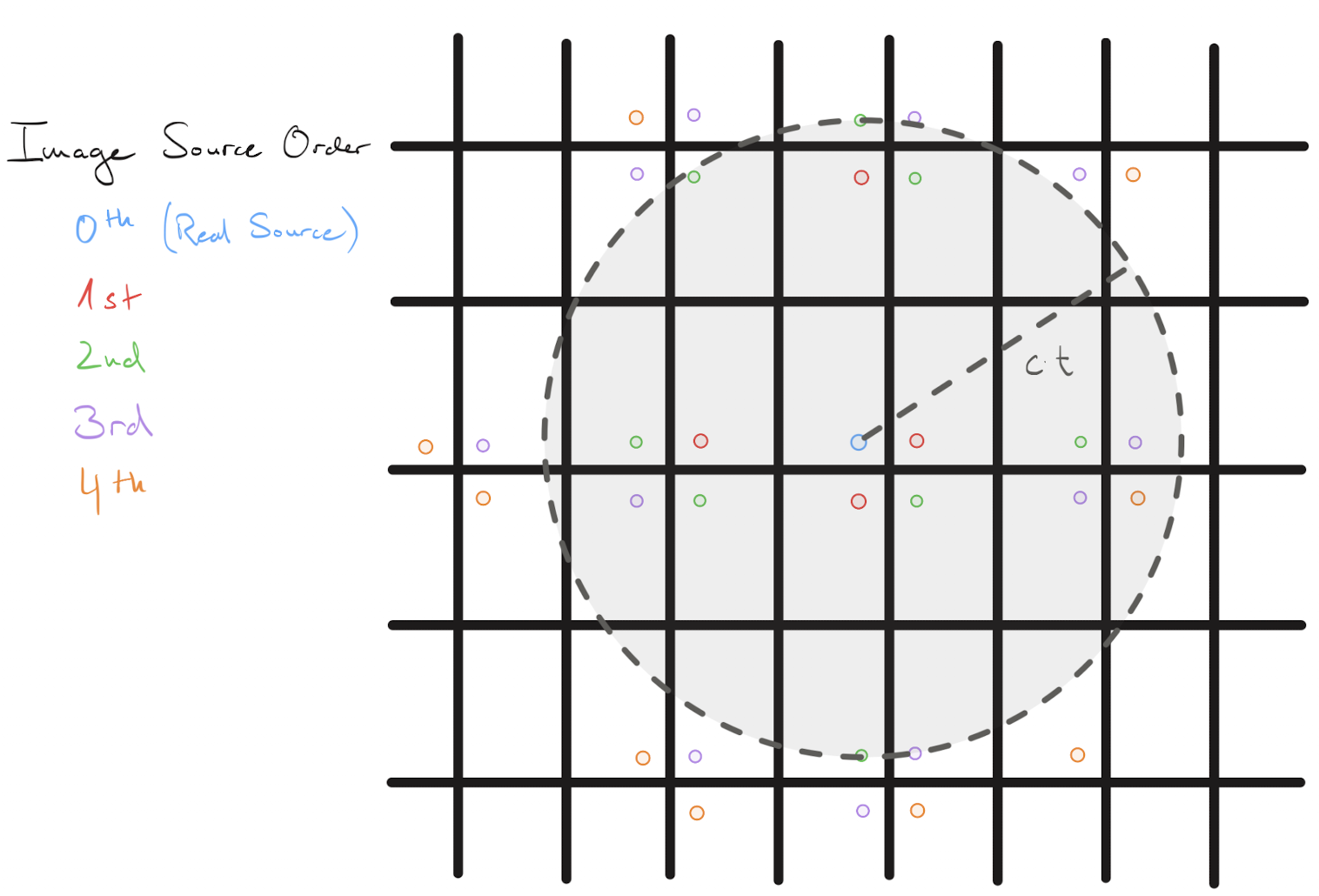
As time evolves, the number of contributing image sources grows rapidly because reflections from more distant mirrored rooms arrive later. Each additional reflection order adds a new “shell” of image rooms in a 3D lattice, so the count of images up to order N grows roughly like O(N^3), see Figure 5.1. If we treat image sources as a uniform lattice with one image per room volume V, then the expected number of images within a propagation radius r = c\,t is proportional to the volume of a sphere: N(t) \approx \frac{\frac{4\pi}{3}(c\,t)^3}{V} \quad .
5.3.5 ISM in Rectangular Rooms
In the implementation for Assignment 4, the image method starts by building an image source index list. We create integer index vectors
\mathbf{i} = (i_x, i_y, i_z) \in \mathbb{Z}^3
and collect all indices whose image source order is within a chosen limit, e.g.,
|i_x| + |i_y| + |i_z| \le N_{\max},
excluding \mathbf{i}=\mathbf{0} (the direct sound). This list is the imageSourceList: each row says how many mirror-room shifts we apply along each axis. In the 2D assignment code the list is \mathbf{i}=(i_x,i_y), built from a grid of indices, sorted by order, and filtered to keep only low-order images.
Given a real source position \mathbf{s} and room dimensions \mathbf{L}=(L_x,L_y,L_z), each image source position is computed by mirroring \mathbf{s} across the room boundaries. The code uses an odd/even rule per axis: \mathbf{s}_\text{img} = \mathbf{i}\odot\mathbf{L} \;+\; \mathbf{b}\odot\mathbf{L} \;+\; (1-2\mathbf{b})\odot\mathbf{s}, where \mathbf{b} = \mathbf{i}\bmod 2 (0 for even, 1 for odd), and \odot is element‑wise multiplication. This matches the idea that even indices repeat the source position, while odd indices flip it inside a mirrored room.
Finally, the room impulse response is assembled by summing the contributions from all image sources. For each image source, compute its distance to the listener r_k = \lVert \mathbf{s}_{\text{img},k} - \mathbf{l} \rVert, apply delay \tau_k = r_k/c, geometric spreading 1/r_k, and (optionally) wall reflection coefficients. In its simplest form, h(t) = \sum_k a_k \, \delta\!\left(t - \frac{r_k}{c}\right), and in the code each image source is passed through a propagation model (delay, attenuation, air absorption) and then summed to produce the early‑reflection response.
5.3.6 Implementation Considerations
When implementing the image method:
- Order limitation: Only compute reflections up to a certain order (typically 1-3 for early reflections)
- Visibility checking: Verify that image sources are “visible” (path doesn’t intersect walls)
- Distance attenuation: Apply 1/r law for geometric spreading
- Air absorption: Apply frequency-dependent air absorption
- Time delays: Compute propagation delays for each reflection
- Spatial rendering: Each reflection arrives from a specific direction
The image method provides an efficient way to generate early reflections, but it has limitations:
- Visibility check is computationally expensive for complicated room geometries
- Assumes specular (mirror-like) reflections
- Doesn’t account for diffraction or scattering
- Becomes computationally expensive for high orders
5.4 Wave Domain Modeling
5.4.1 From Geometric to Wave Acoustics
While geometric acoustics works well for high frequencies and early reflections, wave acoustics is necessary for:
- Low frequencies: When wavelengths are comparable to room dimensions
- Room modes: Resonant frequencies determined by wave interference
- Standing waves: Patterns of constructive and destructive interference
Wave domain modeling solves the wave equation subject to boundary conditions, revealing how sound waves interfere to create room modes. A comparison of geometric and wave acoustics is shown in the video below.
5.4.2 The Wave Equation in Rooms
The wave equation describes how acoustic pressure p(\mathbf{r}, t) evolves in space and time:
\frac{\partial^2 p}{\partial t^2} = c^2 \nabla^2 p
where:
- c is the speed of sound
- \nabla^2 is the Laplacian operator
For a shoebox room with rigid boundaries, we solve this equation subject to:
- Boundary conditions: \frac{\partial p}{\partial n} = 0 at all walls (normal derivative is zero)
- Initial conditions: The sound source excitation
5.4.3 Separation of Variables
For rectangular rooms, we can use separation of variables to find solutions. Assuming a solution of the form:
p(x, y, z, t) = X(x) Y(y) Z(z) T(t)
Substituting into the wave equation and applying boundary conditions yields:
p_{n_x, n_y, n_z}(x, y, z, t) = \cos\left(\frac{n_x \pi x}{L_x}\right) \cos\left(\frac{n_y \pi y}{L_y}\right) \cos\left(\frac{n_z \pi z}{L_z}\right) e^{i \omega_{n_x, n_y, n_z} t}
where (n_x, n_y, n_z) are mode indices (non-negative integers).
5.5 Room Modes and Eigenfrequencies
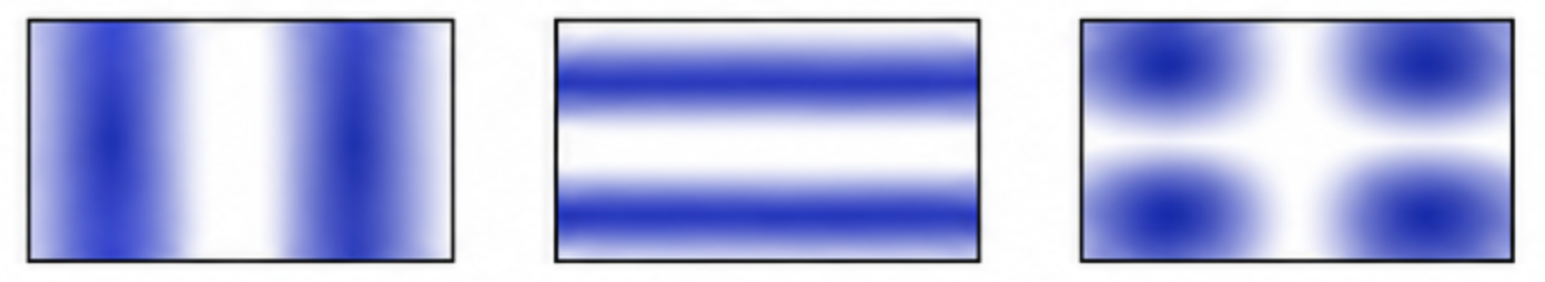
The indices (n_x, n_y, n_z) label standing‑wave room modes and their spatial patterns in a rectangular room. The figure below shows one such mode shape in the plane z=0.
For a shoebox room with rigid boundaries, the angular eigenfrequency \omega_{n_x,n_y,n_z} and the (cyclic) frequency f_{n_x,n_y,n_z} are related by \omega_{n_x,n_y,n_z} = 2\pi f_{n_x,n_y,n_z}, and the eigenfrequencies are:
f_{n_x, n_y, n_z} = \frac{c}{2} \sqrt{\left(\frac{n_x}{L_x}\right)^2 + \left(\frac{n_y}{L_y}\right)^2 + \left(\frac{n_z}{L_z}\right)^2}
5.5.1 Mode Types
Room modes are classified by how many mode indices are non-zero:
- Axial modes (n_x, 0, 0), (0, n_y, 0), (0, 0, n_z): Waves between two parallel walls
- Tangential modes (n_x, n_y, 0), (n_x, 0, n_z), (0, n_y, n_z): Waves involving four walls
- Oblique modes (n_x, n_y, n_z) with all indices non-zero: Waves involving all six walls
Axial modes are typically the strongest and most problematic.
5.5.2 Mode Density
The modal density (number of modes per frequency interval) increases with frequency. At low frequencies, modes are sparse and well-separated. At high frequencies, modes overlap and the response becomes diffuse.
Using the eigenfrequency formula, the number of modes below frequency f is approximately the number of integer lattice points inside a sphere of radius k = \frac{2\pi f}{c} in n‑space. This gives the classical asymptotic count N(f) \approx \frac{4\pi}{3}\frac{V}{c^3} f^3, so the modal density is the derivative n(f) = \frac{\mathrm{d}N}{\mathrm{d}f} \approx \frac{4\pi V}{c^3} f^2.
The Schroeder frequency (or critical frequency) marks the transition: f_c \approx 2000 \sqrt{\frac{T_{60}}{V}}
where T_{60} is the reverberation time and V is the room volume. Above this frequency, the room response is diffuse and statistical methods apply.
5.5.3 Frequency Response
The frequency response of a room shows peaks at eigenfrequencies. The amplitude of each peak depends on:
- Source position: Excites some modes more than others
- Listener position: Some positions are at pressure nodes (minima) or antinodes (maxima)
- Damping: Higher damping reduces peak amplitudes
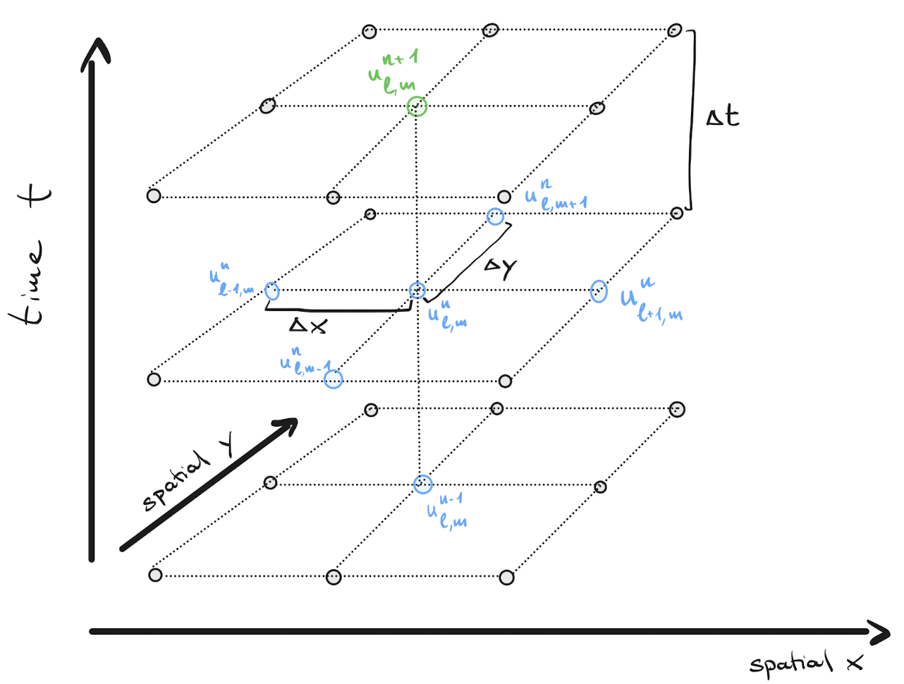
5.5.4 Finite Difference Time Domain (FDTD) in 2D
FDTD solves the wave equation numerically on a grid (instead of the analytic mode solution). For the 2D case, \frac{1}{c^2}\frac{\partial^2 u}{\partial t^2} = \frac{\partial^2 u}{\partial x^2} + \frac{\partial^2 u}{\partial y^2}, we sample the sound pressure field u(x, y, t) on a lattice: u_{l,m}^n \approx u(n\Delta t,\, l\Delta x,\, m\Delta y) and replace derivatives by finite differences. This gives \frac{u_{l,m}^{n+1}-2u_{l,m}^{n}+u_{l,m}^{n-1}}{(c\Delta t)^2} = \frac{u_{l+1,m}^{n}-2u_{l,m}^{n}+u_{l-1,m}^{n}}{(\Delta x)^2} \;+\; \frac{u_{l,m+1}^{n}-2u_{l,m}^{n}+u_{l,m-1}^{n}}{(\Delta y)^2}.
With \Delta x = \Delta y and choosing the time step to satisfy the Courant–Friedrichs–Lewy (CFL) condition—which ensures numerical stability in wave simulations—specifically c\Delta t/\Delta x = \sqrt{1/2}, the interior-node recursion simplifies to u_{l,m}^{n+1}=\tfrac12\!\left(u_{l+1,m}^{n}+u_{l-1,m}^{n}+u_{l,m+1}^{n}+u_{l,m-1}^{n}\right)-u_{l,m}^{n-1}. For rigid walls the boundary condition is \hat{\mathbf{n}}\cdot\nabla u=0; in practice the assignment enforces it by counting the number of interior neighbors K_{l,m} and using the modified update u_{l,m}^{n+1}=\left(2-\tfrac12 K_{l,m}\right)u_{l,m}^{n}+\tfrac12\!\sum_{\text{neighbors}} u^{n}-u_{l,m}^{n-1}, while nodes outside the room are kept at zero. An excellent introduction is given in the tutorial by Brian Hamilton.
Because the grid only resolves wavelengths larger than about 2\Delta x, the excitation must be band‑limited to avoid spatial aliasing and numerical dispersion. The assignment therefore uses a short, smooth one‑period sine (raised‑cosine windowed) or similar band‑limited pulse so that most energy lies below the grid cutoff frequency. A sharp impulse excites high frequencies that the grid cannot represent and produces ringing and unstable‑looking artifacts.
5.6 Summary and Outlook
5.6.1 Key Concepts Covered
In this handbook, we have introduced the fundamental concepts of architectural acoustics:
- Early reflections: Discrete echoes that arrive shortly after direct sound
- Image method: Efficient technique for computing reflections in rectangular rooms
- Room modes: Standing wave patterns at resonant frequencies
- Eigenfrequencies: Frequencies determined by room geometry and boundary conditions
- Wave domain modeling: Solving the wave equation to understand low-frequency behavior
5.6.2 The Complete Room Acoustic Model
A realistic room acoustic model includes:
- Direct sound: Free-field propagation with distance attenuation and air absorption
- Early reflections: Image method for shoebox rooms (up to order 1-3)
- Room modes: Wave domain modeling for low frequencies
- Late reverberation: Statistical or physical modeling (covered in Assignment 5)
5.6.3 Assignment 4 Tasks
Assignment 4 will guide you through:
Part 1: Early Reflections
- Implementing the image method for a shoebox room
- Computing reflection paths and arrival times
- Applying reflection coefficients and attenuation
- Combining direct sound and early reflections with binaural rendering
Part 2: Wave Domain Modeling
- Computing room eigenfrequencies
- Understanding mode shapes and types
- Simulating the wave domain model using FDTD
- Visualizing room modes
5.6.4 Limitations and Extensions
The techniques covered in this assignment have limitations:
- Image method: Only works for rectangular rooms with specular reflections
- Wave domain: Assumes rigid boundaries and simple geometries
- Early reflections: Doesn’t account for diffraction, scattering, or frequency-dependent reflection
Advanced techniques address these limitations:
- Ray tracing: For arbitrary geometries
- Finite element methods: For complex boundary conditions
- Hybrid methods: Combining geometric and wave acoustics
5.6.5 Next Steps
After completing Assignment 4, you will have:
- Understanding of early reflections and room modes
- Tools for modeling simple room acoustics
- Foundation for advanced reverberation techniques
Assignment 5 will build upon these concepts to introduce artificial reverberation algorithms for modeling late reverberation.
5.6.6 Further Reading
Modern acoustic simulation software solves the wave equation using advanced numerical techniques, such as the finite difference method (FDM) and finite element method (FEM). In practice, these wave-based methods are often combined with geometric acoustics to efficiently model both wave phenomena (such as room modes) and specular reflections. For a glimpse into how cutting-edge startups are leveraging these techniques, see this demonstration from Treble Technologies.