PortAudio library not found4 Ambisonics
Lab Handbook - Assignment 3
This handbook provides the theoretical foundation for understanding Ambisonics, a scene-based spatial audio format that uses spherical harmonics to represent sound fields. Ambisonics enables flexible encoding, transmission, and decoding of spatial audio for various playback systems. We will walk step by step from physical sound fields to the math and then to practical encoding/decoding. You do not need advanced acoustics to follow along, but you should be comfortable with basic signals, Fourier ideas, and vector/matrix notation.
The original version of this handbook was created by Chris Hold, Aalto University.
4.1 Table of Contents
4.2 Introduction to Ambisonics
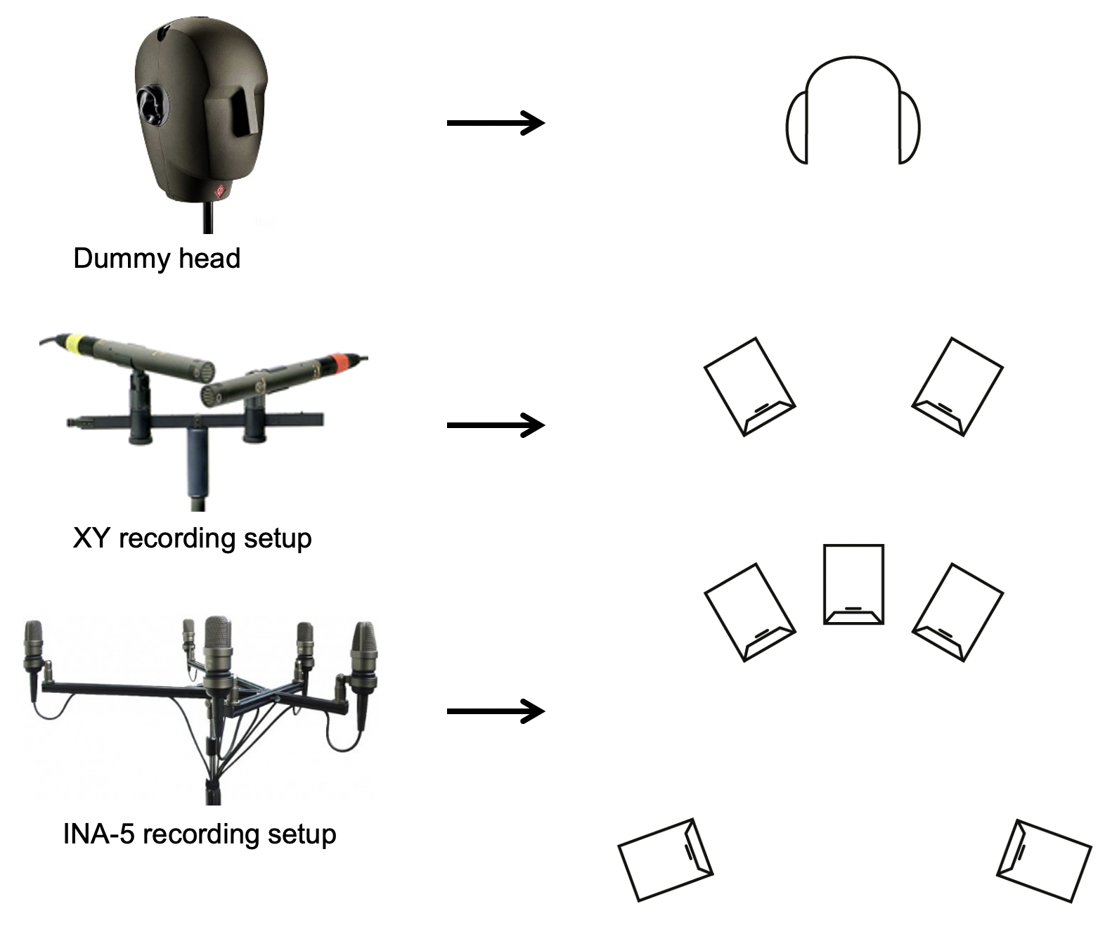
The figure shows a direct progression from capture method to playback format: a dummy‑head recording maps naturally to headphone listening, an XY stereo pair maps to a conventional two‑speaker setup, and a multichannel array like INA‑5 maps to larger loudspeaker layouts. The key point is that traditional recordings are tightly coupled to a specific playback configuration, which limits flexibility when the listening setup changes. Ambisonics breaks that link by capturing the sound field itself, so you can decode later to headphones, stereo, or multi‑speaker arrays without re‑recording.
4.2.1 What is Ambisonics?
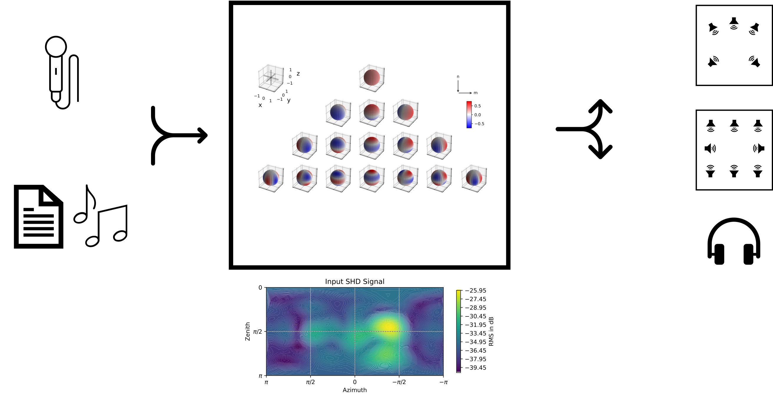
Ambisonics is a scene-based spatial audio format that represents sound fields using spherical harmonics. Unlike channel-based formats (stereo, 5.1) or object-based formats (individual sources with metadata), Ambisonics captures the entire sound field as a continuous function, enabling flexible encoding, transmission, and decoding for various playback systems. In practice this means the recording is not tied to a specific loudspeaker layout. You can record once, store or transmit the Ambisonics coefficients, and later decode them for headphones, a stereo pair, or a full loudspeaker array. In the labs we will treat Ambisonics as a simple pipeline: encode sources, optionally process in the spherical-harmonic domain, then decode.
If you are interested in the artistic applications of Ambisonics, you can check out the Ninth International Student 3D Audio Production Competition.
4.3 Scene-Based Audio Formats
4.3.1 Audio Description Formats
There are three main approaches to spatial audio. Channel-based audio stores signals that already correspond to speakers. Object-based audio stores a set of sources plus metadata that describes where they should be rendered. Scene-based audio stores a complete description of the sound field itself. This difference matters for flexibility: if the playback system changes, a channel-based recording typically needs a new mix, while a scene-based recording can be decoded to the new system without re-authoring. Keep this in mind as you work through the assignments, because the same Ambisonics data can support multiple playback targets.
| Channel Based | Object Based | Scene Based |
|---|---|---|
- Channel Based: Fixed number of channels (e.g., stereo, 5.1, 7.1) with predefined speaker positions
- Object Based: Individual sources with position metadata, rendered at playback time
- Scene Based: Complete sound field representation, independent of playback system
4.3.2 Benefits of Scene-based
- Separation of concerns: Recording, transmission/storage, and playback are independent
- Flexibility: Multiple options for each stage of the pipeline
- Scalability: Does not scale with the number of sources
- Format-agnostic: Same content works for different playback systems
- Rotation-invariant: Easy to rotate sound fields
In short, the scene-based approach keeps your recordings future‑proof: you can postpone the playback decision until the end of the workflow.
4.3.3 Example: Signal Combination
The following example demonstrates how combining signals in the scene-based format works. Because the representation is linear, you can add two sound fields by simply adding their spherical-harmonic representations. For instance two microphones, one with omni pattern and one with figure-of-eight pattern, can be combined to form a cardioid pattern. This property is useful in the labs, where you will build scenes by superposition of multiple sources.

4.4 From Wave Equation to Spherical Harmonics
We start from physics to show where the spherical-harmonic representation comes from, then quickly move to the practical formulas you will use in code. The wave equation is a partial differential equation that describes the propagation of sound waves in a medium. \nabla^2 p - \frac{1}{c^2} \frac{\partial^2 p}{\partial t^2} = 0 \quad.
In frequency domain, with wave-number k = \frac{\omega}{c} the wave equation results in the Helmholtz equation.
(\nabla^2 + k^2) p = 0 \quad.
This separation is valuable because it enables us to analyze each frequency on its own and to use spatial basis functions (like spherical harmonics) for representing the field at that frequency. In laboratory exercises, this is why we process audio in the spherical-harmonic domain on a per-frequency-bin basis.
There are many valid solutions to the wave or Helmholtz equation; for example, a monochromatic plane wave (with amplitude \hat{A}(\omega)) in Cartesian coordinates. Plane waves are particularly useful because any complex sound field can be described as a sum or integral of plane waves from different directions. Ambisonics leverages this by efficiently encoding those directional components in a compact format. p(t, x, y, z) = \hat{A}(\omega) e^{i(k_x x + k_y y + k_z z - \omega t)} \quad.

Any solution to the Helmholtz equation can also be expressed in spherical coordinates. This expansion separates the radial part (how the field behaves with distance) from the angular part (how it varies with direction). For Ambisonics we focus on the angular part on a sphere, which is where spherical harmonics provide an orthonormal basis. p(r, \theta, \phi, k) = \sum_{n = 0}^{\infty} \sum_{m=-n}^{n} \color{olive}{(A_{mn} j_n(kr) + B_{mn} y_n(kr))} \; \color{brown}{Y_{n}^{m}(\theta,\phi)} \quad,
p(r, \theta, \phi, k) = \sum_{n = 0}^{\infty} \sum_{m=-n}^{n} \color{olive}{C_{mn}(kr)} \; \color{brown}{Y_{n}^{m}(\theta,\phi)} \quad,
With two separable parts:
- radial component : linear combination of spherical Bessel functions of first (j_n) and second kind y_n
- angular component : spherical harmonics \color{brown}{Y_{n}^{m}(\theta,\phi)}
A sound field defined on a sphere can be completely described by its spherical harmonics coefficients. In practice, this means you can measure or simulate the pressure values on a sphere and represent them with a finite set of coefficients. The truncation order N determines the amount of directional detail that can be preserved.
E.g. a unit plane wave is given by p(r, \theta, \phi, k) = \sum_{n = 0}^{\infty} \sum_{m=-n}^{n} 4 \pi i^n j_n(kr) \left[ Y_n^m(\theta_k,\phi_k) \right] ^* Y_{n}^ {m}(\theta,\phi) \quad.
4.5 Spherical Harmonics
The Spherical Harmonics represent spatial functions on the sphere and are a spatial version of the Fourier Series, which is a basis for representing periodic functions in the time domain. Instead of the sinusoidal basis functions in the time domain, the spherical harmonics are a basis for representing functions on the sphere.
The spherical harmonics are defined as: Y_n^m(\theta,\phi)=\color{orange}{\sqrt{\frac{2n+1}{4\pi}\frac{(n-m)!}{(n+m)!}}}\, \color{teal}{P_n^m(\cos(\theta))}\, \color{purple}{e^{im\phi}} \quad,
Y_n^m(\theta,\phi)=\color{orange}{D_{nm}}\, \color{teal}{P_n^m(\cos(\theta))}\, \color{purple}{e^{im\phi}} \quad, where
- \phi is the azimuth and \theta is the zenith/colatitude.
- P_n^m is the associated Legendre polynomial of order n and degree m.
Combined with appropriate scaling, the real Spherical Harmonics Y_{n,m}(\theta,\phi) (please note the difference between Y_n^m and Y_{n,m}) are given by
Y_{n,m}(\theta,\phi) = \color{orange}{D_{n|m|}}\, \color{teal}{P_{n}^{|m|}(\cos(\theta))}\, \color{purple}{ \begin{cases} \sqrt2\sin(|m|\phi) & \mathrm{if\hspace{0.5em}} m < 0 \quad,\\ 1 & \mathrm{if\hspace{0.5em}} m = 0 \quad,\\ \sqrt2\cos(|m|\phi) & \mathrm{if\hspace{0.5em}} m > 0 \quad. \end{cases} }
- The definition of spherical harmonics varies across the literature and implementations. For example, it is advisable to always check whether the Condon–Shortley phase convention (-1)^m is used.

The spherical harmonics consist of two separable components:
- Azimuthal component \color{purple}{e^{im\phi}}: Determines the variation in the horizontal plane (azimuth)
- Zenithal component \color{teal}{P_n^m(\cos(\theta))}: Determines the variation in the vertical plane (elevation/zenith)
These components are multiplied together and scaled to create the complete spherical harmonic function. The order n sets the spatial complexity, while the degree m sets the orientation of that pattern around the sphere. You can think of low orders as capturing broad, smooth variations and higher orders as capturing finer angular detail.


4.6 Orthonormality
Two functions \textcolor{violet}{f}, \textcolor{purple}{g} over a domain \gamma are orthogonal if
\int \textcolor{violet}{f^*(\gamma)} \textcolor{purple}{g(\gamma)} \,\mathrm{d}\gamma = \langle \textcolor{violet}{f}, \textcolor{purple}{g} \rangle = 0 \quad,\,\mathrm{for}~f \neq g.
They are also orthonormal if \textcolor{violet}{\int f^*(\gamma) f(\gamma) \,\mathrm{d}\gamma = \int|f(\gamma)|^2 \,\mathrm{d}\gamma = \langle f, f \rangle } = 1 \quad, \\ \textcolor{purple}{\int g^*(\gamma) g(\gamma) \,\mathrm{d}\gamma = \int |g(\gamma)|^2 \,\mathrm{d}\gamma = \langle g, g \rangle} = 1 \quad.
For the spherical harmonics
- the azimuthal component e^{im\phi} along \phi is orthogonal w.r.t. the degree m
- the zenithal component P_n^m(\cos\theta) along \theta is orthogonal w.r.t. the order n.
Their product is still orthogonal, and the scaling \color{orange}{D_{nm}} ensures orthonormality such that the spherical harmonics behave like an energy-preserving basis. This is essential for the encoder and decoder: coefficients can be interpreted as projections, and simple inner products recover the original field (up to truncation). \int_{\mathbb{S}^2} Y_n^m(\Omega)^* \, Y_{n'}^{m'}(\Omega) \,\mathrm{d}\Omega = \langle Y_n^m , Y_{n'}^{m'} \rangle = \delta_{nn'}\delta_{mm'} \quad ,
and
\int_{\mathbb{S}^2} |Y_n^m({\Omega})|^2 \mathrm{d}{\Omega} = 1 \quad .
4.7 Spherical Harmonic Transform
Our goal is to find a scene based encoding for sound fields.
- We showed that the spherical harmonics Y_n^m({\Omega}) are a set of suitable basis functions on the sphere
- We also showed that a sound field (on the sphere) s({\Omega}) is fully captured by its spherical harmonics coefficients \sigma_{nm}
This can be expressed with \Omega = [\phi, \theta] as the inverse Spherical Harmonic Transform (iSHT). The iSHT reconstructs a directional sound field from a finite set of coefficients, which is exactly what a decoder does when it generates loudspeaker or binaural signals. s({\Omega}) = \sum_{n = 0}^{N=\infty} \sum_{m=-n}^{+n} \sigma_{nm} Y_n^m({\Omega}) \quad.
Spherical harmonics coefficients \sigma_{nm} can be derived with the Spherical Harmonic Transform (SHT). In the labs you will implement this idea with discrete measurements, which turns the integral into a weighted sum over sample points on the sphere. \sigma_{nm} = \int_{\mathbb{S}^2} s({\Omega}) [Y_n^m({\Omega})]^* \mathrm{d}{\Omega} = \langle [Y_n^m] , s) \rangle \quad.
- SHT is also referred to as spherical Fourier transform.
- Note the transform is between a spatially continuous and a discrete frequency domain. This is similar to the Discrete Time Fourier Transform (DTFT), which transforms a discrete time signal into a continuous frequency domain signal.
4.8 Spherical Grids
The SHT evaluates the continuous integral over \Omega. In practice we only sample the sphere at a finite set of points, so the grid you pick matters for accuracy. \sigma_{nm} = \int_{\mathbb{S}^2} s({\Omega}) [Y_n^m({\Omega})]^* \mathrm{d}{\Omega} \quad . Quadrature methods allow evaluation by spherical sampling at certain (weighted) grid points such that \sigma_{nm} \approx \sum_{q=1}^{Q} w_q s({\Omega}_q) [Y_n^m({\Omega}_q)]^* \quad.
Certain grids with sampling points {\Omega}_q and associated sampling weights w_q have certain properties. The grid choice affects how accurately you can represent a sound field of a given order. In practice you need at least (N+1)^2 well-distributed points and appropriate weights to avoid bias in the coefficients.
- quadrature grids allow numerical integration of spherical polynomials
- Spherical sampling dictates maximum order
- easy to evaluate are uniform/regular grids, with constant w_q = \frac{4\pi}{Q}
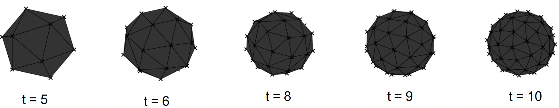
- An example are so-called spherical t-designs(t), which allow a SHT up to order N = \lfloor t/2 \rfloor

4.9 Spherical Dirac
We can show that spherical harmonics are orthogonal (even orthonormal) with \int_{\mathbb{S}^2} Y_n^m(\Omega) \, Y_{n'}^{m'}(\Omega) \,\mathrm{d}\Omega = \delta_{nn'}\delta_{mm'} \quad .
Because of their completeness, we can also directly formulate a Dirac function on the sphere as a sum of spherical harmonics. This is a useful theoretical tool: it explains why a single plane wave can be encoded by evaluating the basis at one direction, and it motivates beamforming as a directional filter in the spherical-harmonic domain. \sum_{n=0}^{N=\infty} \sum_{m=-n}^n [Y_n^m({\Omega'})]^* Y_n^m(\Omega) = \delta(\Omega - \Omega') \quad,
and therefore the spherical Fourier coefficients \sigma_{nm} SHT\{\delta(\Omega - \Omega')\} = \int_{\mathbb{S}^2} \delta(\Omega - \Omega') \, [Y_n^m({\Omega})]^* \mathrm{d}{\Omega} = [Y_n^m({\Omega'})]^* \quad .
4.10 Order-Limitation of Spherical Dirac Pulse
In a finite-order system the Dirac impulse cannot be perfectly sharp. The plot below shows how the main lobe tightens as order increases, which is the same resolution trade‑off you will see in decoding.

4.10.1 Example
Integrate (order-limited) Dirac \delta_N(\Omega - \Omega') over sphere
\int_{\mathbb{S}^2} \delta_N(\Omega - \Omega') \mathrm{d}{\Omega} = \int_{\mathbb{S}^2} \color{blue}{\sum_{n=0}^{N} \sum_{m=-n}^n\, [Y_n^m({\Omega'})]^* Y_n^m(\Omega)} \,\mathrm{d}{\Omega} \quad,
by discretization with sufficient t-design \int_{\mathbb{S}^2} \color{blue}{\sum_{n=0}^{N} \sum_{m=-n}^n\, [Y_n^m({\Omega'})]^* Y_n^m(\Omega)} \,\mathrm{d}{\Omega} = \frac{4\pi}{Q}\sum_{q=1}^{Q} \color{orange}{\sum_{n=0}^{N} \sum_{m=-n}^n\, [Y_n^m({\Omega'})]^* Y_n^m(\Omega_q)}

4.11 Matrix Notations
To implement the pipeline efficiently, it helps to write everything in matrix form. The next few lines introduce the standard stacking used in Ambisonics toolkits. Stack the spherical harmonics evaluated at \Omega up to spherical order N as
\mathbf{Y} = \left[ \begin{array}{ccccc} Y_0^0(\Omega[0]) & Y_1^{-1}(\Omega[0]) & Y_1^0(\Omega[0]) & \dots & Y_N^N(\Omega[0]) \\ Y_0^0(\Omega[1]) & Y_1^{-1}(\Omega[1]) & Y_1^0(\Omega[1]) & \dots & Y_N^N(\Omega[1]) \\ \vdots & \vdots & \vdots & \vdots & \vdots \\ Y_0^0(\Omega[Q-1]) & Y_1^{-1}(\Omega[Q-1]) & Y_1^0(\Omega[Q-1]) & \dots & Y_N^N(\Omega[Q-1]) \end{array} \right]
such that \mathbf{Y} is of size Q \times (N+1)^2
soundfield pressure is real signal -> only real spherical harmonics needed
orthonormal scaling introduced earlier called N3D by convention (in contrast to SN3D)
stacking them as above, where \mathrm{idx}_{n,m} = n^2+n+m, is called ACN
We can stack a time signal s(t_0, t_1, \ldots, t_T) as vector \mathbf{s}. \mathbf{s} = \begin{bmatrix} s(t_0) \\ s(t_1) \\ \vdots \\ s(t_T) \end{bmatrix}
This leads to a matrix notation of multiple discrete signals \mathbf{S} of size T \times Q. \mathbf{S} = \begin{bmatrix} s_0(t_0) & s_1(t_0) & \cdots & s_Q(t_0)\\ s_0(t_1) & s_1(t_1) & \cdots & s_Q(t_1)\\ \vdots & \vdots& \ddots & \vdots \\ s_0(t_T) & s_1(t_T) & \cdots & s_Q(t_T) \end{bmatrix}
Similarly, stacking Ambisonics coefficients \sigma_n^m(t_0, t_1, \ldots, t_T) into \mathbf{\chi} of size T \times (N+1)^2 \mathbf{\chi} = \begin{bmatrix} \sigma_0^0(t_0) & \sigma_1^{-1}(t_0) & \cdots & \sigma_N^N(t_0) \\ \sigma_0^0(t_1) & \sigma_1^{-1}(t_1) & \cdots & \sigma_N^N(t_1) \\ \vdots & \vdots & \ddots & \vdots \\ \sigma_0^0(t_T) & \sigma_1^{-1}(t_T) & \cdots & \sigma_N^N(t_T) \end{bmatrix}
We obtain ambisonic signals matrix \mathbf{\chi} of size T \times (N+1)^2 from signals \mathbf{S} of size T \times Q by SHT in matrix notation as \mathbf{\chi} = \mathbf{S} \, \mathrm{diag}(w_q) \, \mathbf{Y} \quad. With the SH basis functions evaluated at \Omega_q as \mathbf{Y} of size Q \times (N+1)^2.
Obtaining the discrete signals s_q(t) is a linear combination of SH basis functions evaluated at \Omega_q. This inverse SHT in matrix notation is
\mathbf{S} = \mathbf{\chi} \, \mathbf{Y}^T \quad .
From the Ambisonics Encoder, to Directional Weighting, to a Decoder, the same linear algebra structure appears repeatedly. Writing the operations in matrix form makes it easier to implement and to reason about computational cost, and it highlights that most steps are linear transforms.
4.12 Ambisonics Encoder
A single plane wave encoded in direction \Omega_1 with signal \mathbf{s} is directly the outer product with the Dirac SH coefficients. Intuitively, the direction selects the spherical-harmonic basis weights, and the signal supplies the time variation. Multiple sources then add linearly, which is why the encoder is often a simple weighted sum, i.e.,
\mathbf{\chi}_\mathrm{PW(\Omega_1)} = \mathbf{s} \, \mathbf{Y}(\Omega_1) \quad.
For multiple sources Q, we stack and sum \mathbf{\chi}_\mathrm{PW(\Omega_Q)} = \sum_{q=1}^Q\mathbf{s}_q \, \mathbf{Y}(\Omega_q) = \mathbf{S} \, \mathbf{Y} \quad.


4.13 Directional Weighting
- Directionally filtering a soundfield in direction \Omega_k by weighting
- Weighting in SH domain w_{nm} is an elegant way of beamforming
The simplest beamformer is a spherical Dirac in direction \Omega_k normalized by its energy, i.e., \mathrm{max}DI. More advanced beamformers trade off sharpness and robustness, and they can be implemented by applying order-dependent weights to the coefficients. You will explore these patterns to see how they affect spatial selectivity. w_{nm, \mathrm{maxDI}}(\Omega_k) = \frac{4\pi}{(N+1)^2} Y_{n,m}(\Omega_k)

Other patterns can be achieved by weighting the spherical Fourier spectrum. Axis-symmetric patterns reduce to only a modal weighting c_n, such that w_{nm}(\Omega_k) = c_{n} \, Y_{n,m}(\Omega_k)
E.g. \mathrm{max}\vec{r}_E weights each order n with c_{n,\,\mathrm{max}\vec{r}_E} = P_n[\cos(\frac{137.9^\circ}{N+1.51})] \quad, with the Legendre polynomials P_n of order n.

In the assignment, you will be implementing the beamformer based on \mathrm{max}\vec{r}_E.
4.14 Ambisonics Decoder
Decoding turns the Ambisonics coefficients back into signals you can listen to. You can think of it as steering a set of beamformers toward a set of target directions. These decoders are called Sampling Ambisonics Decoders (SAD).
- Beamformer extracts a portion of the soundfield in steering direction \Omega
- Pointing a set of beamformers in directions \Omega_k results in a set of signal components
- in case of \mathrm{max}DI proportional to iSHT in \Omega_k
x({\Omega_k}) = \sum_{n = 0}^{N} \sum_{m=-n}^{+n} w_{nm}({\Omega_k}) \, \sigma_{nm} \quad,
or in matrix notation with \mathbf{X} and beamforming weights \mathbf{c}_n and \mathbf{Y} \mathbf{X} = \mathbf{\chi} \, \mathrm{diag_N}(\mathbf{c}_n) \, \mathbf{Y}^T \quad .

4.14.1 Example


4.14.2 Example
Decode on a t-design(6) (sufficient up to N = 3):
- a 3rd order ambisonic signal
- a 5th order ambisonic signal
- an 8th order ambisonic signal


4.15 Loudspeaker Decoding
Different decoder algorithms can be used for loudspeaker playback. The choice of decoder impacts energy distribution, localization accuracy, and robustness to irregular loudspeaker layouts. In the labs you will compare these strategies qualitatively and observe how order and array geometry influence the results.
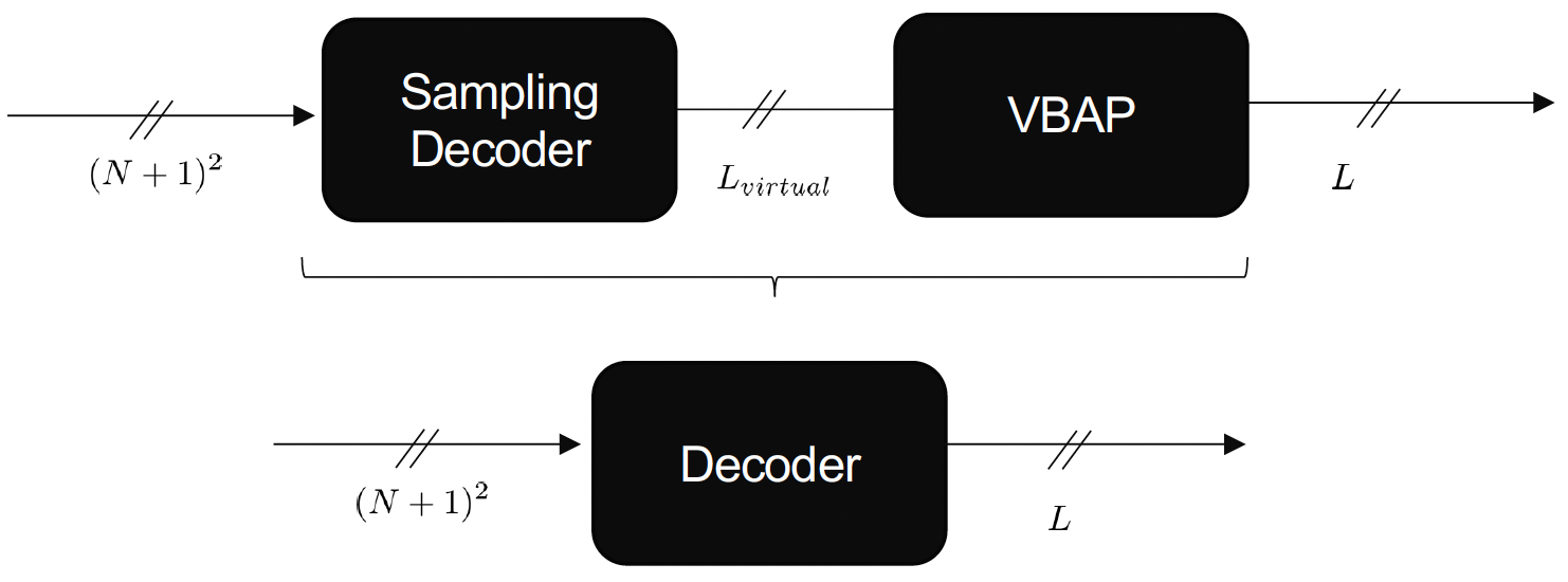
AllRAD (All‑Round Ambisonic Decoding) can be understood as SAD plus a panning stage: first decode the Ambisonics signal to a dense set of virtual loudspeakers on a spherical t‑design (standard SAD), then re‑render those virtual signals to the actual loudspeaker layout using VBAP/triangulation. This keeps SAD’s stable soundfield sampling while adapting to irregular or sparse real arrays.
Face not pointing towards listener: [0 1 2]
Face not pointing towards listener: [0 6 2]
Face not pointing towards listener: [2 5 6]
Face not pointing towards listener: [2 3 4]
Face not pointing towards listener: [2 5 4]


4.16 Binaural Decoding
For headphones, we use head‑related impulse responses (HRIRs) to recreate directional cues. The key idea is that each Ambisonics component is filtered and summed to form the left and right ear signals.
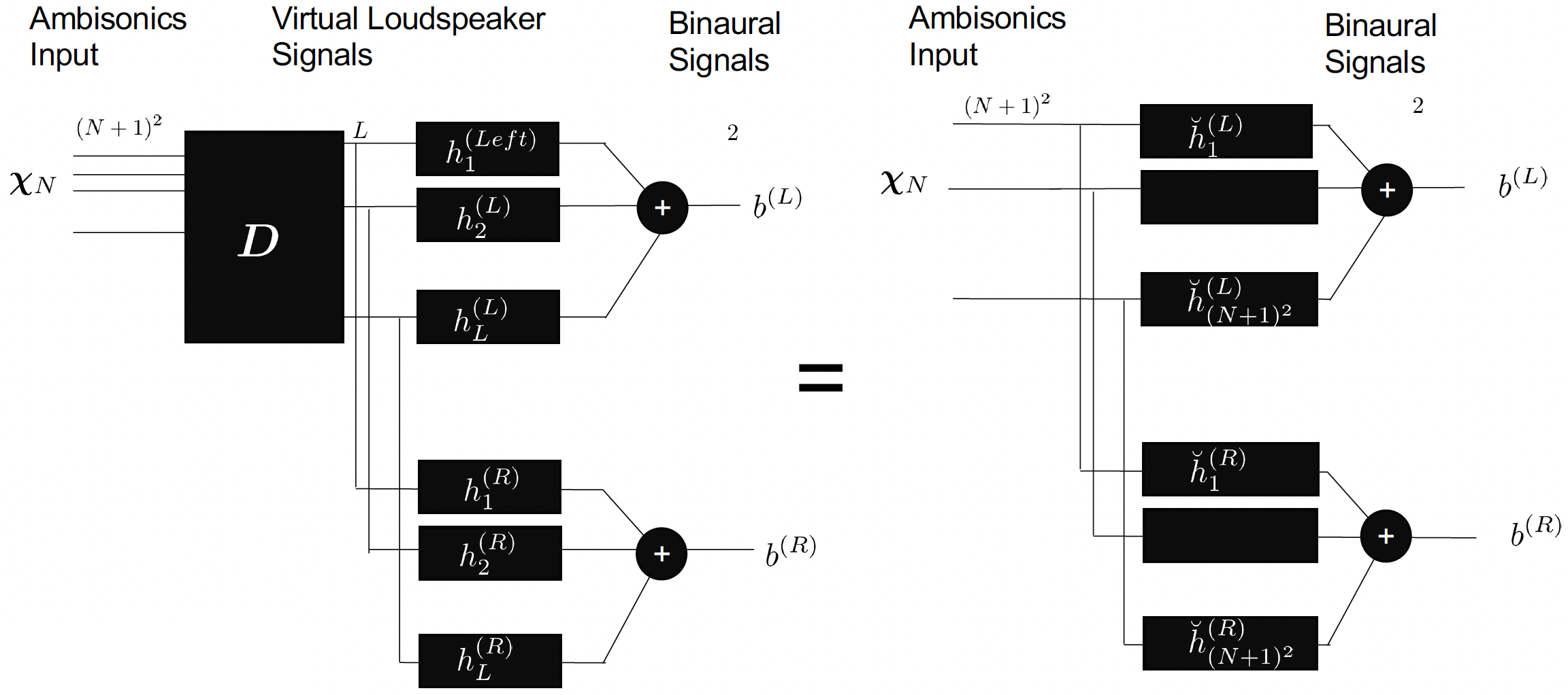
b^{L,R}(t) = x(t) * h_{\mathrm{HRIR}}^{L,R}({\Omega}, t) \quad, where (*) denotes the time-domain convolution operation.
Transforming to the time-frequency domain through the time-domain Fourier transform, further assuming plane-wave components \bar X (\Omega), the ear input signals are given as B^{L,R}(\omega) = \int_{\Omega} \bar X (\Omega, \omega) H^{L,R}(\Omega, \omega) \,\mathrm{d}\Omega \quad.
B^{L,R}(\omega) = \sum_{n = 0}^{N} \sum_{m = -n}^{+n} \chi_{nm}(\omega) \breve H_{nm}^{L,R}(\omega) \quad.
For one ear (left) this can be interpreted as a frequency dependent ambisonic beamformer b^L(\omega) = \chi_{nm}(\omega) [\breve H_{nm}^{L}(\omega)]^T \quad .
4.17 Summary and Outlook
You now have the building blocks needed for the lab tasks. The list below is a quick checklist of what you should be comfortable with before moving on.
4.17.1 Key Concepts Covered
In this handbook, we have introduced the fundamental concepts of Ambisonics:
- Scene-based audio: Flexible format separating recording, transmission, and playback
- Spherical harmonics: Orthonormal basis functions on the sphere
- Spherical Harmonic Transform (SHT): Converting between spatial and frequency domains
- Ambisonics encoding: Representing sound sources as spherical harmonic coefficients
- Ambisonics decoding: Reconstructing sound fields for loudspeaker or binaural playback
- Ambisonic order: Trade-off between spatial resolution and channel count
4.17.2 The Complete Ambisonics Pipeline
An Ambisonics system consists of:
- Encoding: Converting source signals and directions to Ambisonic coefficients
- Processing: Optional manipulation in the spherical harmonic domain
- Decoding: Converting Ambisonic coefficients to loudspeaker signals or binaural audio
4.17.3 Assignment 3 Tasks
Assignment 3 will guide you through:
- Evaluating spherical harmonics: Understanding the basis functions
- Implementing the encoder: Converting sources to Ambisonic format
- Implementing loudspeaker decoder: Reconstructing sound fields for loudspeaker arrays
- Implementing binaural decoder: Creating spatialized audio for headphones
- Exploring Ambisonic orders: Understanding how order affects spatial resolution
4.17.4 Ambisonic Order
The Ambisonic order N determines:
- Spatial resolution: Higher orders provide better angular resolution
- Channel count: (N+1)^2 channels required
- Frequency range: Higher orders needed for higher frequencies
- Computational cost: Increases with order
Common orders:
- First order (N=1): 4 channels (B-format), basic spatial audio
- Third order (N=3): 16 channels, good spatial resolution
- Fifth order (N=5): 36 channels, high spatial resolution
4.17.5 Advantages of Ambisonics
- Format-agnostic: Same content works for different playback systems
- Rotation-invariant: Easy to rotate sound fields
- Scalable: Can truncate to lower orders if needed
- Efficient: Compact representation of sound fields
- Flexible: Supports various decoding strategies
4.17.6 Limitations
- Order limitation: Finite order limits spatial resolution
- Frequency-dependent: Higher orders needed at higher frequencies
- Decoder-dependent: Quality depends on decoder design
- Loudspeaker setup: Requires appropriate loudspeaker configurations
4.17.7 Next Steps
After completing Assignment 3, you will have:
- Understanding of Ambisonics encoding and decoding
- Tools for creating spatial audio content
- Foundation for advanced spatial audio techniques
Future assignments will build upon these concepts to include room acoustics modeling and artificial reverberation.