6 Artificial Reverberation
Lab Handbook - Assignment 5
This handbook provides the theoretical foundation for understanding artificial reverberation algorithms, focusing on Feedback Delay Networks (FDNs) for modeling late reverberation. These techniques are essential for creating realistic and musically pleasing reverberation effects in virtual acoustics and audio production.
6.1 Table of Contents
6.2 Introduction to Artificial Reverberation
6.2.1 What is Reverberation?
Reverberation (often shortened to “reverb”) is the persistence of sound in an enclosed space after the original sound source has stopped. It results from sound waves reflecting off surfaces multiple times, creating a dense, diffuse sound field that decays over time.
Reverberation is a crucial component of room acoustics:
- Early reflections: Discrete echoes arriving within the first 50-100 ms (covered in Assignment 4)
- Late reverberation: Dense, diffuse sound field from many overlapping reflections (covered in this assignment)
6.2.2 Why Artificial Reverberation?
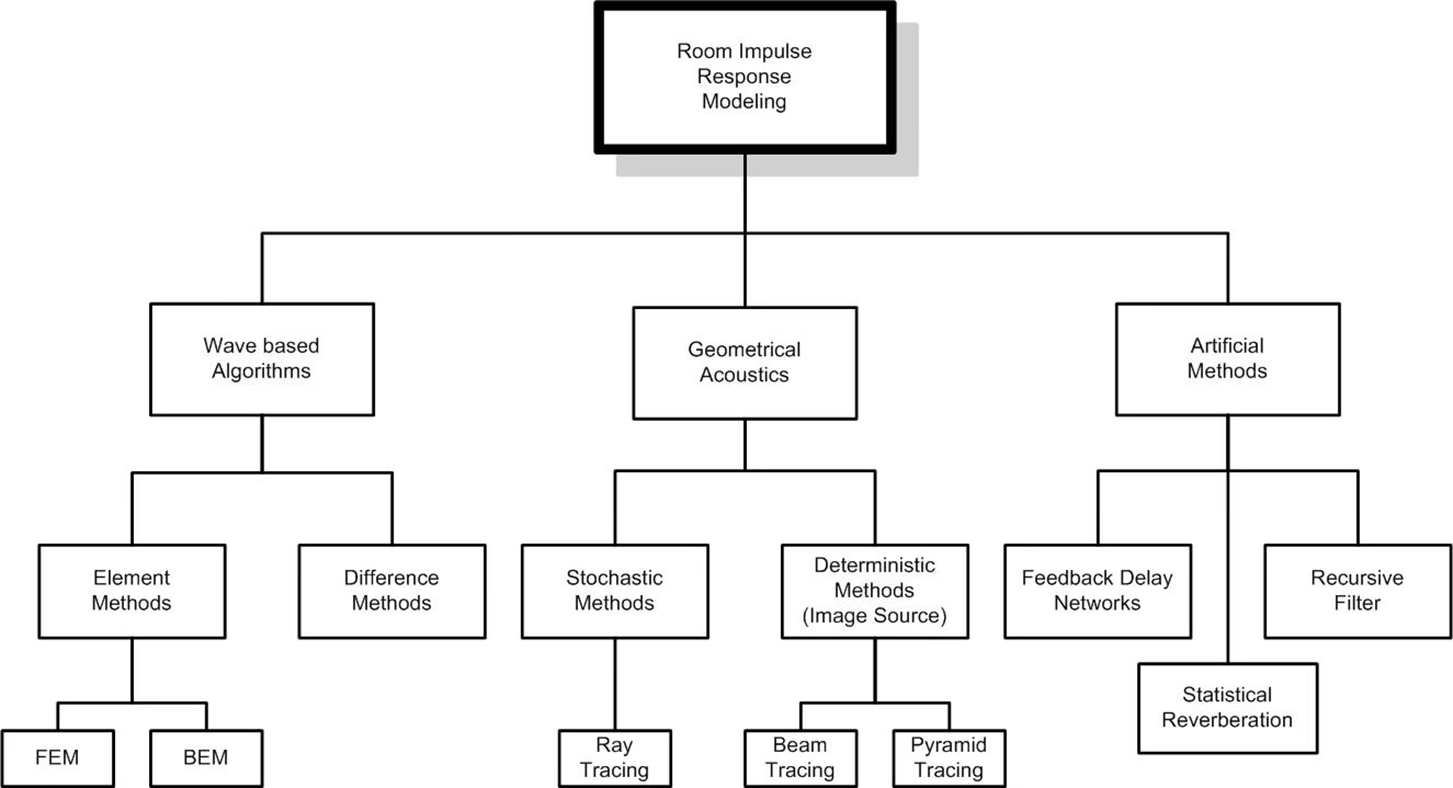
While physical modeling of reverberation (using ray tracing, image methods, or wave equation solvers) can be accurate, it is often:
- Computationally expensive: Requires significant processing power
- Difficult to control: Parameters are tied to physical properties
- Limited flexibility: Hard to achieve specific aesthetic goals
Artificial reverberation algorithms provide:
- Efficient computation: Real-time processing on modest hardware
- Musical control: Parameters can be adjusted for artistic purposes
- Flexibility: Can create effects that don’t exist in nature
- Consistency: Predictable and repeatable results
6.2.3 Applications
Artificial reverberation is used in:
- Music production: Adding space and depth to recordings. See excellent blog posts by Valhalla DSP.
- Virtual acoustics: Creating realistic acoustic environments such as MPEG-I by Fraunhofer IIS and others.
- Gaming: Enhancing immersion and spatial awareness such as Wwise Spatial Audio.
- Virtual reality: Providing acoustic context for virtual spaces such as Meta Audio SDK.
- Live sound: Enhancing performances with reverb effects. For example, L-Acoustics Active Acoustics System Ambience and LMS Acoustics Lab
- Audio post-production: Matching dialogue to scene acoustics. For example, we have developed the reverb behind SpaceLab Interstellar.
6.2.4 Historical Context
The development of artificial reverberation has evolved through several eras:
- Chamber reverb: Using actual rooms or chambers
- Plate and spring reverbs: Mechanical devices (1950s-1970s)
- Digital algorithms: Schroeder’s all-pass and comb filters (1960s)
- Modern algorithms: Feedback Delay Networks, convolution reverb (1980s-present)
This assignment focuses on Feedback Delay Networks (FDNs), which represent the state-of-the-art in artificial reverberation algorithms.
6.3 Reverberation Time and Decay
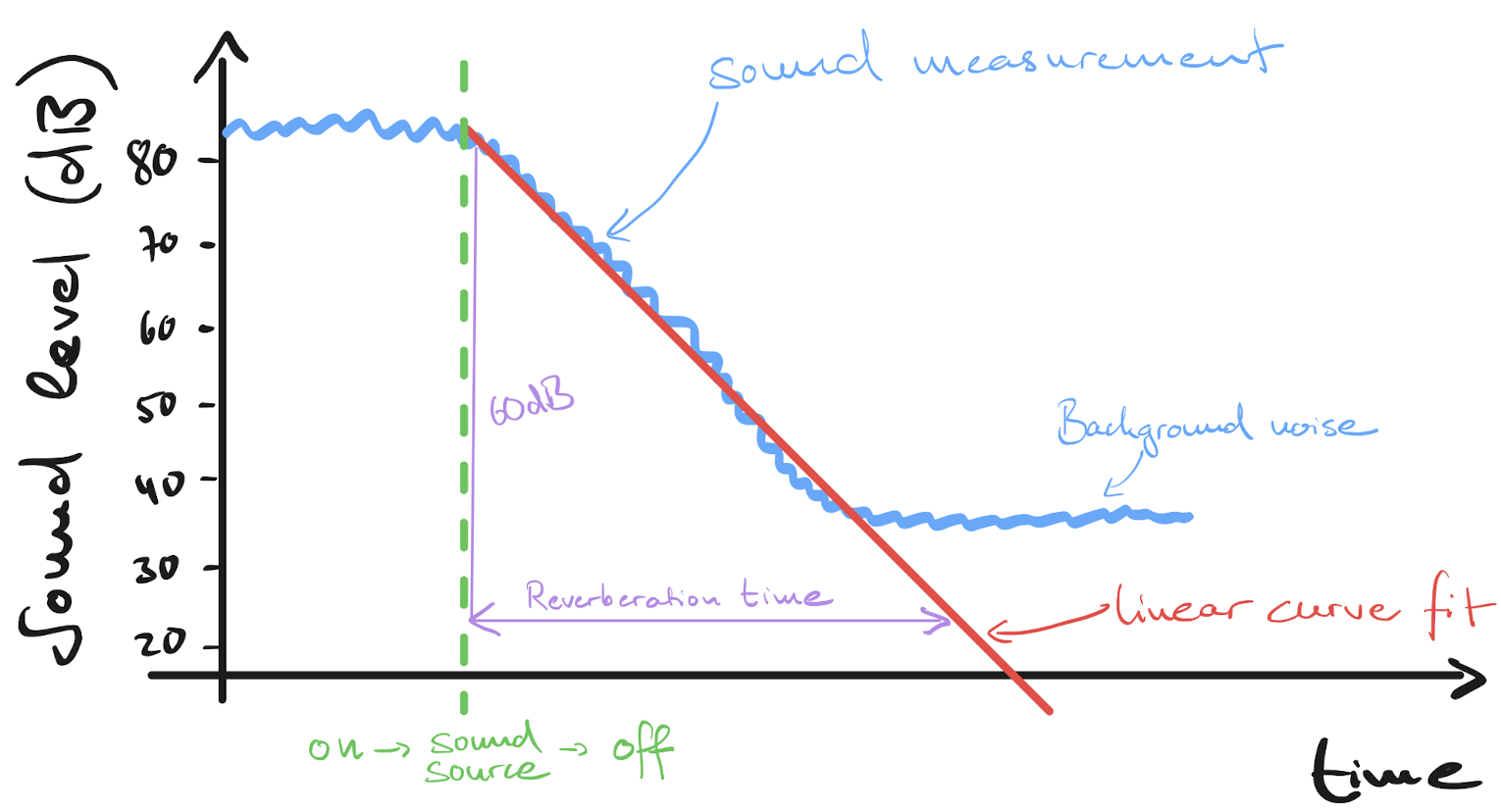
6.3.1 Reverberation Time (RT60)
The reverberation time (RT60 or T60) is the time required for the sound pressure level to decrease by 60 dB after the sound source stops. It is one of the most important parameters characterizing room acoustics. You can listen different room impulse responses with different RT60 values at OpenAir.
6.3.2 Sabine’s Formula
For a room with volume V and total absorption A, Sabine’s formula provides an estimate of reverberation time:
T_{60} = \frac{0.161 \cdot V}{A}
where:
- V is the room volume in cubic meters
- A = \sum_i \alpha_i S_i is the total absorption in square meters (Sabins), where \alpha_i is the absorption coefficient of the i-th surface and S_i is the surface area of the i-th surface.
This formula assumes:
- Diffuse sound field
- Uniform absorption distribution
- Statistical behavior (many reflections)
6.3.3 Frequency-Dependent Reverberation Time
In real rooms, reverberation time varies with frequency:
- Low frequencies: Often longer RT60 (less absorption)
- Mid frequencies: Typically moderate RT60
- High frequencies: Often shorter RT60 (more absorption, air absorption)
This frequency dependence is crucial for realistic reverberation. A good reverb algorithm should allow independent control of RT60 at different frequencies.
6.3.4 Exponential Decay
Reverberation decay is approximately exponential:
p(t) = p_0 \cdot e^{-t/\tau}
where:
- p(t) is the pressure at time t
- p_0 is the initial pressure
- \tau is the decay time constant
The relationship between decay time constant and RT60 is:
\tau = \frac{T_{60}}{6 \ln(10)} \approx \frac{T_{60}}{13.82}
6.3.5 Decay Rate
The decay rate (in dB per second) is:
\text{Decay Rate} = \frac{60}{T_{60}} \text{ dB/s}
In digital systems, we often work with decay per sample:
\text{Decay per sample} = \frac{-60}{T_{60} \cdot f_s} \text{ dB/sample}
where f_s is the sampling rate.
6.4 Delay-Based Reverberation
6.4.1 Basic Concept
Delay-based reverberation algorithms use delay lines (buffers that store past samples) to create echoes and reflections. By feeding delayed signals back into the system, we create multiple echoes that decay over time.
6.4.2 Comb Filters
A comb filter is the simplest delay-based reverb structure. It consists of a delay line with feedback:
y[n] = x[n] + g \cdot y[n-m]
where:
- m is the delay length in samples
- g is the feedback gain (|g| < 1 for stability)
The transfer function is:
H(z) = \frac{1}{1 - g z^{-m}}
6.4.2.1 Frequency Response
The frequency response of a comb filter has peaks (resonances) at frequencies where the delayed signal reinforces the input:
f_k = \frac{k \cdot f_s}{m}, \quad k = 0, 1, 2, \ldots
These peaks create a “comb” pattern in the frequency response, hence the name.
6.4.2.2 Decay Time
The decay time of a comb filter depends on the feedback gain:
T_{60} = \frac{-60 m}{20 \log_{10}(|g|) \cdot f_s}
For a given desired RT60 and delay length m, we can solve for the required gain:
|g| = 10^{-60 m / (20 T_{60} f_s)} = 10^{-3 m / (T_{60} f_s)}
6.4.2.3 Limitations
Simple comb filters have limitations:
- Colored frequency response: Peaks and notches create unnatural sound
- Periodic echoes: Can sound metallic or artificial
- Limited control: Few parameters to adjust
6.4.3 All-Pass Filters
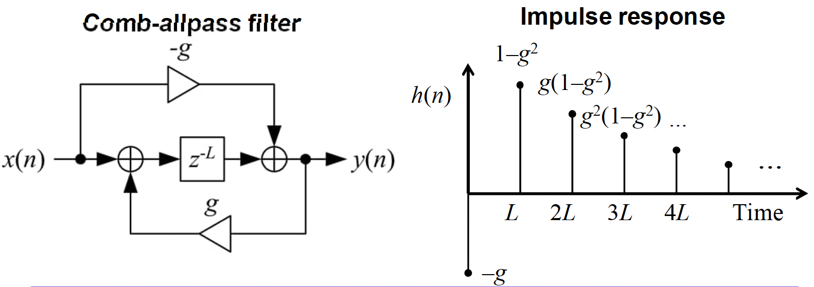
An all-pass filter has a flat magnitude response but introduces phase shifts. It’s useful for decorrelating signals and creating more diffuse reverberation.
A delay-based all-pass filter with delay length L has the form:
H(z) = \frac{-g + z^{-L}}{1 - g z^{-L}}
where g is the all-pass coefficient.
All-pass filters are often cascaded or used in parallel with comb filters to create more complex reverberation patterns.
6.4.4 Schroeder’s Algorithm
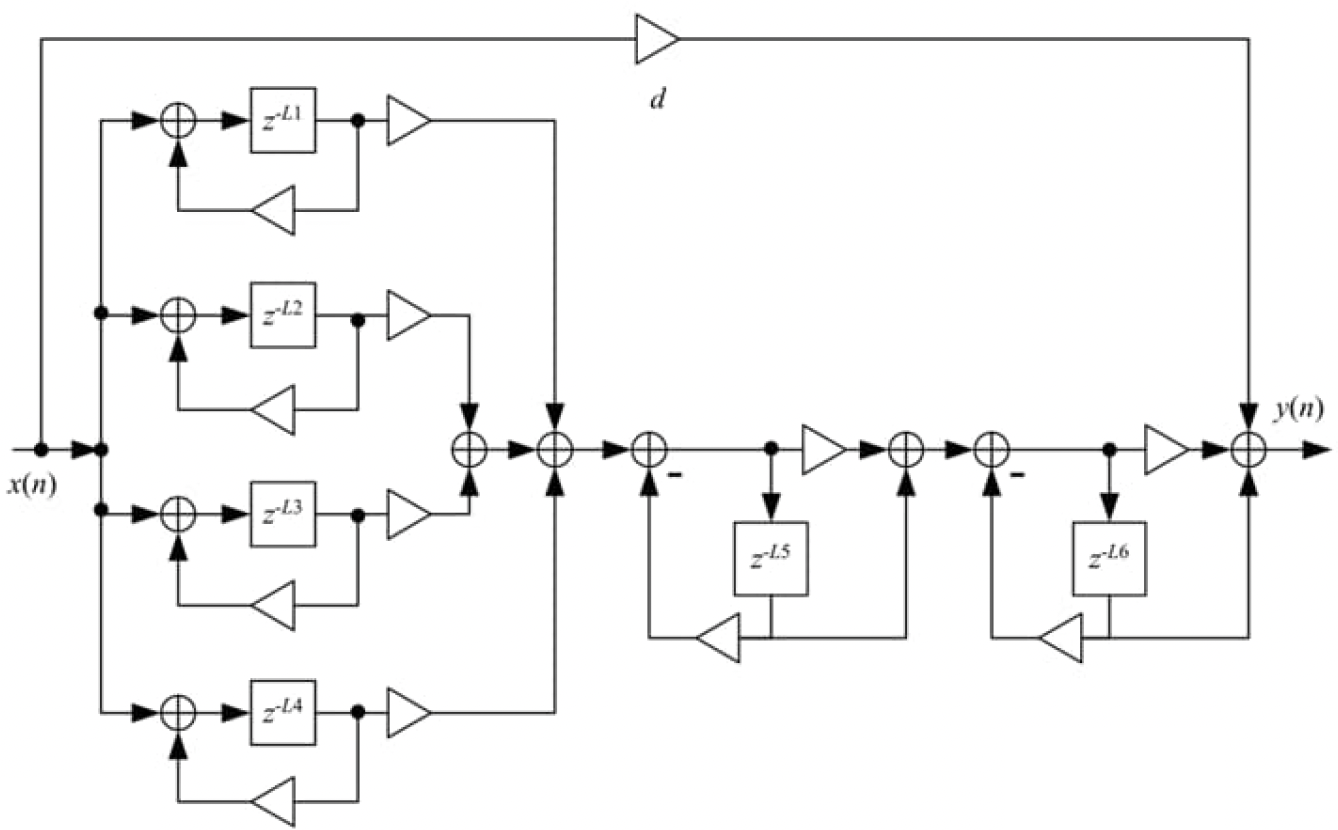
Manfred Schroeder (1962) proposed combining multiple comb filters and all-pass filters:
- Parallel comb filters: Create multiple decay patterns
- Cascaded all-pass filters: Add diffusion and smooth the response
This structure became the foundation for many early digital reverb algorithms.
6.5 Feedback Delay Networks
6.5.1 Introduction to FDNs
Feedback Delay Networks (FDNs) are a generalization of Schroeder’s algorithm that use a feedback matrix to mix multiple delay lines. FDNs were introduced by Gerzon (1972) and further developed by Jot and Chaigne (1991) and represent the state-of-the-art in artificial reverberation.
An FDN consists of:
- Multiple delay lines: Typically 4-16 parallel delay lines
- Feedback matrix: Mixes the outputs of delay lines back to inputs
- Absorption filters: Frequency-dependent attenuation in each delay line
- Input/output gains: Control how signals enter and leave the network
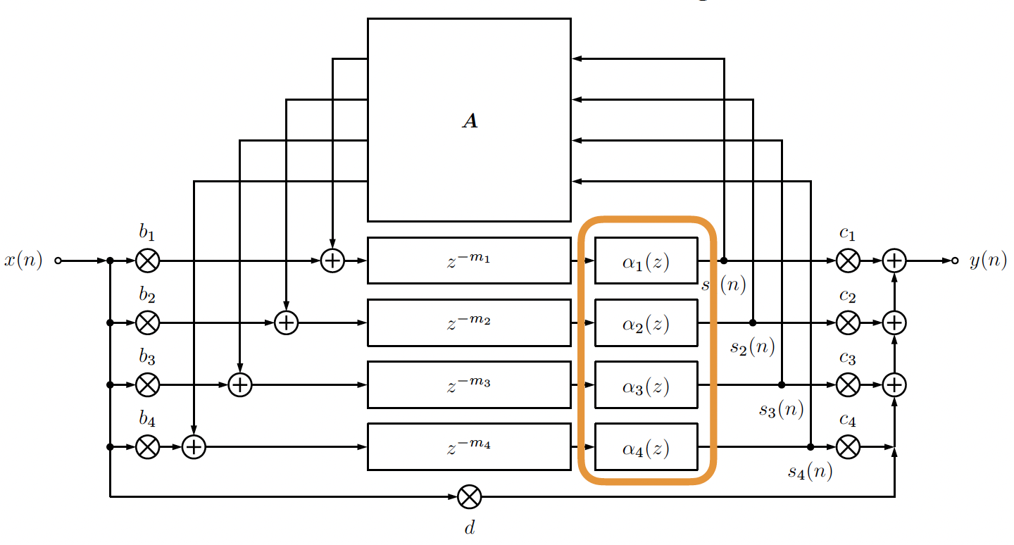
6.5.2 FDN Structure
The FDN can be expressed in delay state-space form as: \begin{align*} \mathbf{s}[n + \mathbf{m}] &= \mathbf{\Gamma} \mathbf{A} \mathbf{s}[n] + \mathbf{B} \mathbf{x}[n] \\ \mathbf{y}[n] &= \mathbf{C} \mathbf{s}[n] + \mathbf{D} \mathbf{x}[n] \end{align*} where:
- \mathbf{s}[n] is the state vector (the contents of the delay lines at time n),
- \mathbf{x}[n] is the input vector,
- \mathbf{y}[n] is the output vector,
- \mathbf{A} is the feedback matrix,
- \mathbf{\Gamma} is a diagonal matrix of attenuation or absorption filters,
- \mathbf{B} and \mathbf{C} are input and output gain matrices,
- \mathbf{D} is the direct path matrix (often zero),
- \mathbf{m} is the vector of delay lengths.
6.5.3 Feedback Matrix
The feedback matrix \mathbf{A} is crucial for FDN performance. It should:
- Be unitary: Preserve energy (orthogonal matrix)
- Create diffusion: Mix signals to avoid periodic patterns
- Be efficient: Allow fast matrix-vector multiplication
Common choices include:
- Hadamard matrix: Orthogonal matrix with \pm 1 entries
- Householder matrix: Reflection-based orthogonal matrix
- Random orthogonal matrix: Generated using QR decomposition
A unitary matrix satisfies:
\mathbf{A}^T \mathbf{A} = \mathbf{I}
This ensures that the FDN is lossless (energy-preserving) when absorption filters are removed.
6.5.4 Delay Lengths
The delay lengths in an FDN should be:
- Mutually prime: Avoid periodic patterns and beating
- Well-distributed: Cover a range of values
- Appropriately scaled: Match the desired room size
Common strategies:
- Prime numbers: Use prime delays to ensure mutual primeness
- Irrational ratios: Use delays related by irrational numbers (e.g., golden ratio)
- Room-based: Calculate delays based on room dimensions
6.5.5 Stability
An FDN is stable if all poles of the system are inside the unit circle. For a lossless FDN (no absorption and marginally stable) the feedback matrix must be unitary. Adding absorption filters to a lossless FDN ensures stability.
6.6 Absorption Filters
6.6.1 Frequency-Dependent Absorption
In real rooms, absorption varies with frequency. To model this realistically, each delay line in an FDN should have a frequency-dependent absorption filter \alpha_i(z).
The absorption filter should:
- Match RT60 curve: Provide desired decay time at each frequency T_{60}(\omega)
- Be efficient: Low computational cost
- Be stable: Guarantee system stability
6.6.1.1 Delay-Proportional Absorption
For delay-proportional absorption, the filter gain |\alpha_i(e^{j\omega})| at frequency \omega depends on the delay length m_i. Longer delays require more attenuation to achieve the same reverberation time.
The relationship is for the i-th delay line:
|\alpha_i(e^{j\omega})| = 10^{-60 m_i / (20 T_{60}(\omega) f_s)}
This ensures that regardless of delay length, the overall decay time is T_{60}(\omega).
6.6.2 One-Pole Absorption Filters
A one-pole filter is a simple and efficient choice for the absorption filter \alpha_i(z) with the transfer function:
H(z) = \frac{b_0}{1 + a_1 z^{-1}}
The frequency response is:
H(e^{j\omega}) = \frac{b_0}{1 + a_1 e^{-j\omega}}
6.6.2.1 Design for Desired RT60
To design a one-pole filter for a specific RT60 at a given delay length m:
Compute desired gain at DC (0 Hz) and Nyquist (f_s/2): H_\text{DC} = 10^{-60 m / (20 T_\text{60,DC} f_s)} H_\text{Nyq} = 10^{-60 m / (20 T_\text{60,Nyq} f_s)}
Solve for filter coefficients a_1 and b_0:
- At DC: H(1) = \frac{b_0}{1 + a_1} = H_\text{DC}
- At Nyquist: H(-1) = \frac{b_0}{1 - a_1} = H_\text{Nyq}
Solve the system: a_1 = \frac{H_\text{DC} - H_\text{Nyq}}{H_\text{DC} + H_\text{Nyq}} b_0 = H_\text{DC} (1 + a_1)
6.6.3 Higher-Order Filters
While one-pole filters are efficient, higher-order filters can provide:
- Better frequency response matching: More accurate RT60 curves
- More control: Independent control at multiple frequencies
- Smoother response: Avoid sharp transitions
Common approaches:
- Second-order sections (SOS): Cascade of biquad filters
- Shelving filters: Low- and high-shelf filters
- Parametric EQ: Multiple bands with independent control
6.6.4 Air Absorption Modeling
In addition to surface absorption, air absorption affects high frequencies. This can be modeled by:
- High-frequency emphasis in absorption filters
- Separate air absorption filter in the signal path
- Frequency-dependent RT that decreases with frequency
6.7 Quality Trade-offs
The following table demonstrates the trade-offs between different FDN configurations:
| Mean Delay (samples) | N = 4 | N = 8 | N = 16 |
|---|---|---|---|
| ~260 | |||
| ~860-900 | |||
| ~2600 |
Key observations:
- Longer delays: More modes, but less echo density
- More delays: Higher modal and echo density, but more computationally expensive
- Feedback matrix: Random orthogonal feedback matrix ensures proper energy distribution
6.8 Digital Signal Processing Implementation
6.8.1 Block-Based Processing
Like other virtual acoustics algorithms, FDNs should use block-based processing:
- Efficient: Process multiple samples at once
- Real-time capable: Low latency
- Compatible: Works with other audio processing
Typical block sizes: 64-1024 samples (256 is common).
6.8.2 Circular Buffers
Delay lines are implemented using circular buffers (ring buffers):
- Efficient: O(1) read/write operations
- Memory efficient: Fixed memory usage
- Simple: Easy to implement
A circular buffer uses:
- Buffer array: Stores delayed samples
- Write index: Current write position
- Read index: Computed as (\text{write} - \text{delay}) \bmod \text{buffer\_size}
6.8.3 Matrix-Vector Multiplication
The feedback matrix multiplication can be optimized:
- Sparse matrices: Sparse matrices can be stored and multiplied efficiently
- Structured matrices: Hadamard matrices have fast algorithms
- SIMD: Vectorized operations for speed
For small FDNs (4-8 delay lines), direct matrix multiplication is usually fast enough.
6.8.4 Filter Implementation
Absorption filters can be implemented as:
- Direct form I/II: Standard IIR filter structures
- Second-order sections: For higher-order filters
- State-space: For numerical stability
6.8.5 Stability Considerations
To ensure stability:
- Check feedback matrix: Should be unitary (or close)
- Verify filter gains: All should be < 1 in magnitude
- Monitor output: Detect and prevent overflow
- Use appropriate data types: Floating-point for accuracy
6.8.6 Parameter Interpolation
For time-varying reverberation (e.g., moving sources), parameters must be interpolated:
- RT60 changes: Smooth absorption filter updates
- Room size changes: Smooth delay length changes
- Crossfading: May be needed for major parameter changes
6.9 Summary and Outlook
6.9.1 Key Concepts Covered
In this handbook, we have introduced the fundamental concepts of artificial reverberation:
- Reverberation time (RT60): Time for sound to decay 60 dB
- Comb filters: Simple delay-based reverb structures
- Feedback Delay Networks (FDNs): Advanced reverb algorithm using multiple delays and feedback matrix
- Absorption filters: Frequency-dependent attenuation for realistic decay
- Trade-offs: Understanding the impact of different FDN configurations
6.9.2 The Complete Reverberation Pipeline
A realistic reverberation system includes:
- Direct sound: Unprocessed source (from Assignment 1)
- Early reflections: Image method for discrete echoes (from Assignment 4)
- Late reverberation: FDN for dense, diffuse tail (Assignment 5)
These components work together to create convincing acoustic environments.
6.9.3 Assignment 5 Tasks
Assignment 5 will guide you through:
- Designing absorption filters: One-pole filters for delay-proportional absorption
- Implementing comb filters: Understanding basic delay-based reverb
- Building an FDN: Complete Feedback Delay Network implementation
- Parameter control: Adjusting RT60, room size, and other parameters
- Integration: Combining with direct sound and early reflections
6.9.4 Advanced Topics
Beyond basic FDNs, advanced techniques include:
- Frequency-dependent scattering feedback matrices: Additional diffusion stages
- Modulated delays and feedback matrices: Chorus-like effects for smoother reverb
- Directional reverberation: Multi-channel FDNs for surround sound
- Physical parameterization: Design FDNs based on physical properties of the room
- Hybrid methods: Combining algorithmic and physical modeling
6.9.5 Next Steps
After completing Assignment 5, you will have:
- Understanding of artificial reverberation algorithms
- Tools for creating realistic and musical reverb
- Foundation for advanced audio effects
6.9.6 Further Reading
For deeper understanding, consider exploring:
- 50 Years of Artificial Reverberation by Välimäki et al. (2012).
- FDN Toolbox by Sebastian J. Schlecht: MATLAB toolbox implementing a wide range of Feedback Delay Network variants and analysis methods for artificial reverberation and decorrelation, including feedback matrix designs, absorption filters, modal decomposition, and allpass filters (github.com/SebastianJiroSchlecht/fdnToolbox). A Python version of the FDN Toolbox is coming soon.