3 Spatial Audio Rendering
Lab Handbook - Assignment 2
This handbook provides the theoretical foundation for understanding spatial audio rendering techniques, focusing on binaural rendering with Head-Related Transfer Functions (HRTFs) and Vector Base Amplitude Panning (VBAP) for loudspeaker arrays.
3.1 Table of Contents
3.2 Introduction to Spatial Audio Rendering
3.2.1 Overview
Spatial audio rendering is the process of delivering audio signals to listeners in a way that creates the illusion of sound sources positioned in three-dimensional space. Unlike the free-field propagation covered in Assignment 1, spatial audio rendering focuses on how sound is delivered to the listener through headphones or loudspeaker arrays.
There are two main approaches to spatial audio rendering:
- Binaural rendering: Uses Head-Related Transfer Functions (HRTFs) to create spatialized audio for headphone playback. To experience binaural rendering, you can watch the Virtual Barber Shop Demo (Youtube video).
- Loudspeaker array rendering: Uses techniques such as VBAP (Vector Base Amplitude Panning) to position virtual sources using multiple loudspeakers. This approach forms the basis for technologies like Dolby Atmos (Dolby Atmos technology) and immersive audio systems used in venues such as the Las Vegas Sphere (Las Vegas Sphere Immersive Audio).
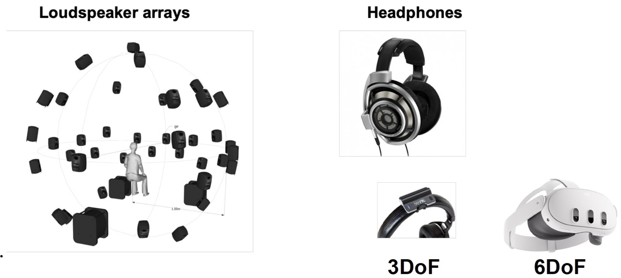
3.2.2 Binaural vs. Loudspeaker Rendering
Binaural rendering advantages:
- Accurate spatial localization for individual listeners
- Works with standard headphones
- Can reproduce complex spatial audio scenes
- No need for specialized loudspeaker setups
Loudspeaker array rendering advantages:
- Natural listening experience (no headphones required)
- Multiple listeners can experience the same spatial audio
- Can create physical sound sources in space
- Suitable for shared listening environments
3.2.3 The Rendering Pipeline
A complete spatial audio rendering system typically involves:
- Source signals: Monophonic or multichannel audio signals
- Spatialization: Applying spatial cues (direction, distance, etc.)
- Rendering: Converting spatialized signals to output format (binaural or loudspeaker signals)
- Playback: Delivering signals to headphones or loudspeakers
In Assignment 2, we explore both binaural rendering with HRTFs and loudspeaker array rendering with VBAP, and how they can be combined.
3.3 Binaural Hearing and HRTFs
3.3.1 How We Localize Sound
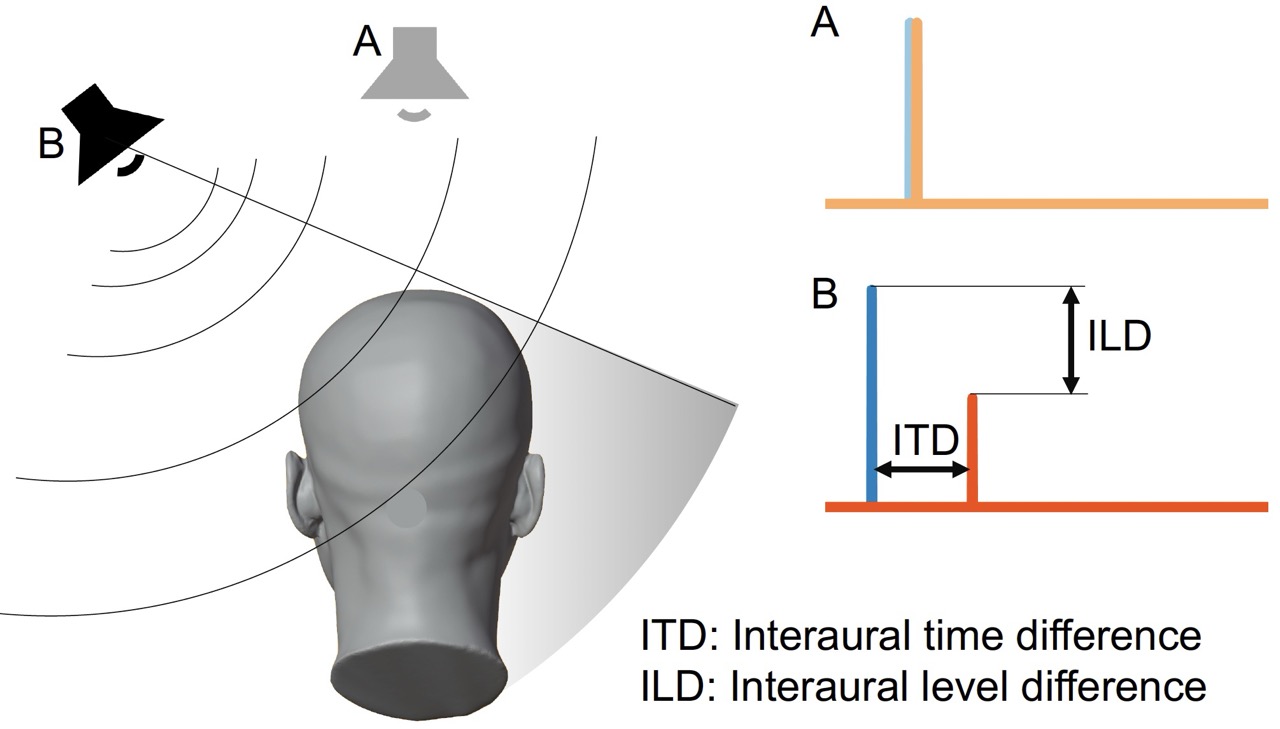
Humans localize sound sources using several acoustic cues:
- Interaural Time Difference (ITD): The difference in arrival time of sound at the left and right ears
- Interaural Level Difference (ILD): The difference in sound level (amplitude) between the left and right ears
- Spectral cues: Frequency-dependent filtering caused by the head, torso, and outer ears (pinnae)
- Head movement: Dynamic cues from head rotation
These cues are captured by Head-Related Transfer Functions (HRTFs), which describe how sound from a specific direction is filtered before reaching the eardrums.
3.3.4 Key Characteristics of HRTFs
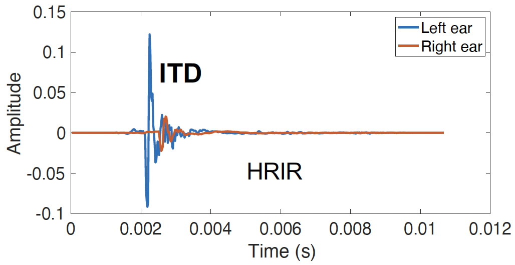
ITD in HRTFs:
- ITD manifests as a time delay between left and right HRIRs
- For sources to the left, the left ear HRIR leads the right ear HRIR
- Typical ITD range: 0 to ~0.7 ms (depending on head size)
- ITD is most effective for frequencies below ~1500 Hz
ILD in HRTFs:
- ILD manifests as amplitude differences between left and right HRTFs
- The head creates a “shadow” effect, attenuating sound at the far ear
- ILD increases with frequency (head shadowing is frequency-dependent)
- Most effective for frequencies above ~1500 Hz
Spectral cues:
- Pinnae (outer ears) create frequency-dependent notches and peaks
- These cues are critical for elevation perception
- Highly individual-specific
3.3.5 HRTF Measurement
HRTFs are typically measured using:
- Dummy heads: Artificial heads with microphones in the ear canals
- Human subjects: Using probe microphones in real ears
- Acoustic simulation: Numerical modeling of head and torso acoustics
Measurements are usually performed on a spherical or dense grid of directions, stored in formats like SOFA (Spatially Oriented Format for Acoustics).
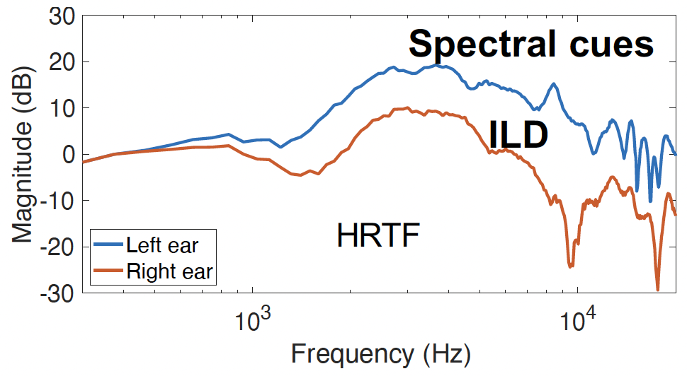
HRTF of left and right ear at azimuth 60 degrees, elevation 30 degrees, distance 1 m. Source: P. Llado.
3.3.6 HRTF Interpolation
Since HRTFs are measured at discrete directions, interpolation is needed for arbitrary source positions. Common approaches include:
- Nearest neighbor: Use the closest measured HRTF (simple but may cause artifacts)
- Barycentric interpolation: Interpolate based on triangular regions
- Spherical harmonic interpolation: Represent HRTFs in spherical harmonic domain
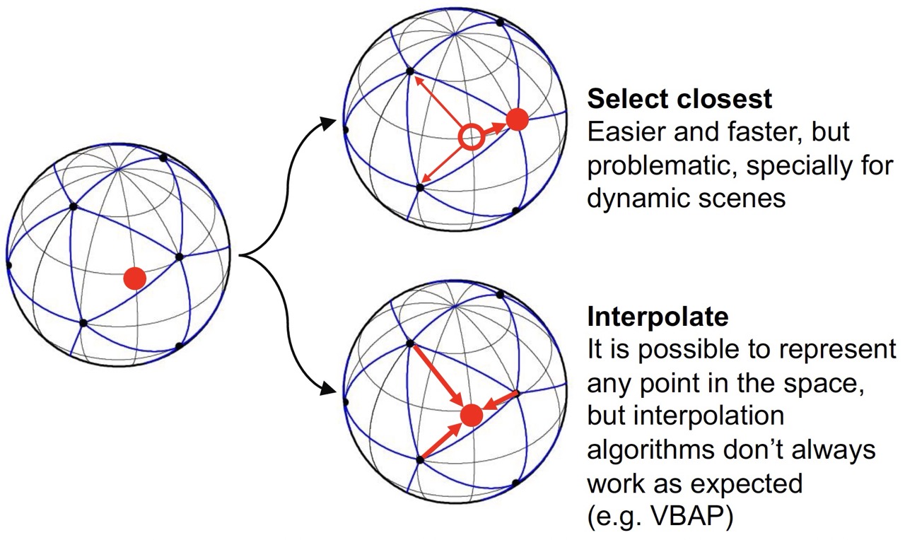
For Assignment 2, we use the nearest neighbor approach for simplicity.
3.4 Binaural Rendering
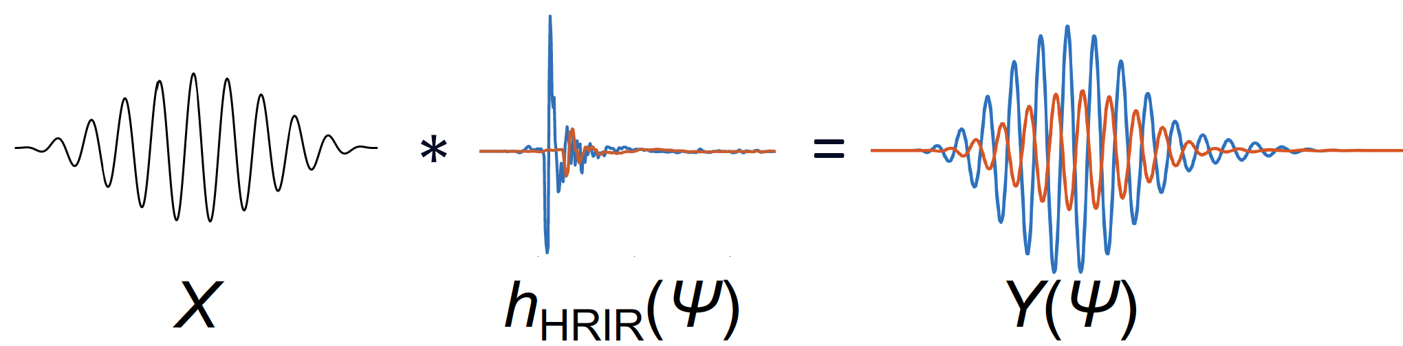
3.4.1 The Binaural Rendering Process
Binaural rendering creates spatialized audio by convolving a monophonic source signal with the appropriate HRIRs for the desired source direction:
y_L[n] = x[n] * h_L[n]
y_R[n] = x[n] * h_R[n]
where:
- x[n] is the source signal
- h_L[n] and h_R[n] are the left and right HRIRs for the source direction
- y_L[n] and y_R[n] are the binaural output signals
3.4.2 Multiple Sources
For multiple sources at different directions, the binaural signals are summed:
y_L[n] = \sum_{i=1}^{N} x_i[n] * h_{L,i}[n]
y_R[n] = \sum_{i=1}^{N} x_i[n] * h_{R,i}[n]
where N is the number of sources and h_{L,i}[n], h_{R,i}[n] are the HRIRs for source i.
3.4.3 Block-Based Convolution
In real-time systems, convolution is performed block-by-block using efficient algorithms:
Overlap-Add Method:
- Divide input signal into blocks
- Convolve each block with the HRIR (using FFT for efficiency)
- Overlap and add the results to handle the “tail” of the convolution
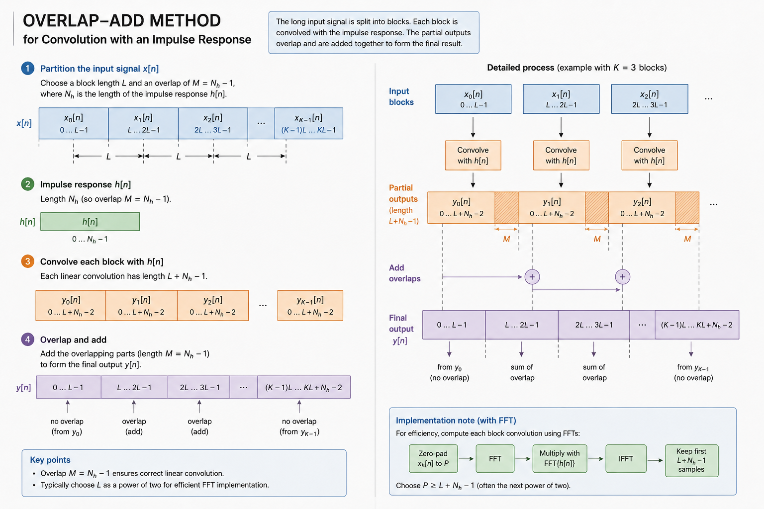
This approach allows for:
- Efficient computation using FFT-based convolution
- Time-varying HRIRs (sources can move)
- Low latency processing
3.4.4 Diffuse Field Equalization
HRTFs measured in anechoic conditions may not sound natural when used for binaural rendering. Diffuse field equalization compensates for this by:
- Computing the average magnitude response across all directions (diffuse field response)
- Designing an inverse filter to flatten this average response
- Applying this filter to all HRIRs
This ensures that a diffuse sound field (like natural room acoustics) is reproduced correctly.
3.4.5 HRTF Selection
For a given source direction (\theta, \phi), we need to select the appropriate HRIRs. The process involves:
- Convert to Cartesian coordinates: Transform spherical coordinates to unit vectors
- Find nearest measurement: Compute angular distance to all measured HRIR positions
- Select HRIRs: Use the HRIRs from the nearest measurement point
The angular distance between two unit vectors \mathbf{p}_1 and \mathbf{p}_2 is:
\alpha = \arccos(\mathbf{p}_1 \cdot \mathbf{p}_2)
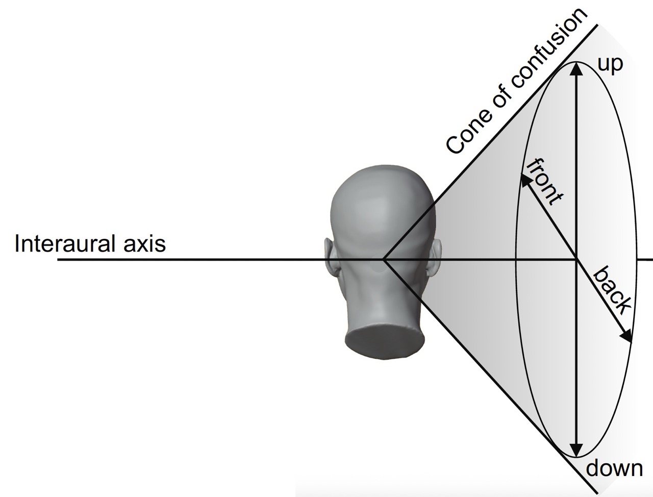
3.4.6 Limitations of Binaural Rendering
- Individual differences: HRTFs are person-specific; using someone else’s HRTFs may reduce localization accuracy
- Front-back confusion: Listeners may confuse sounds in front with sounds behind
- Elevation perception: Can be challenging, especially with non-individualized HRTFs
- Head movement: Static HRTFs don’t account for head rotation (though this can be addressed with head tracking)
3.5 Loudspeaker Array Rendering
3.5.1 Overview
Loudspeaker array rendering positions virtual sound sources using multiple loudspeakers. Unlike binaural rendering, this approach creates physical sound sources in space, making it suitable for shared listening environments.
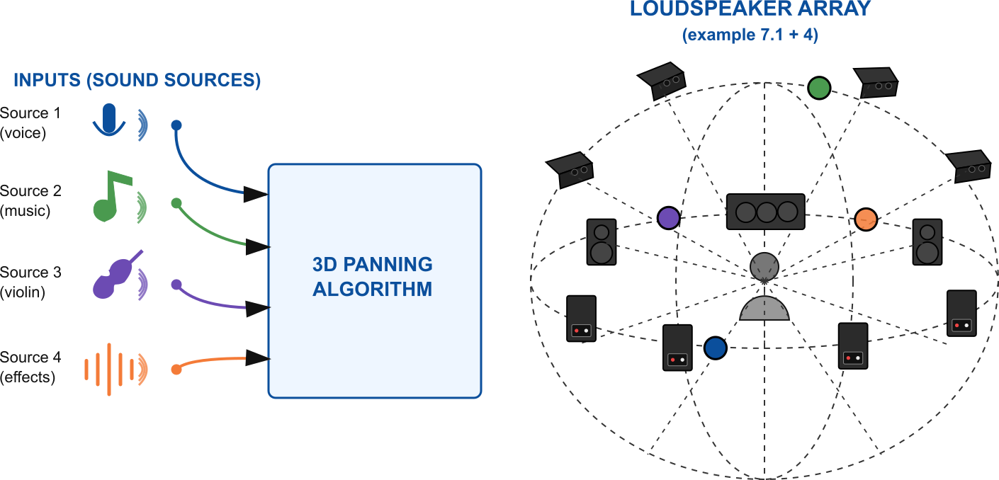
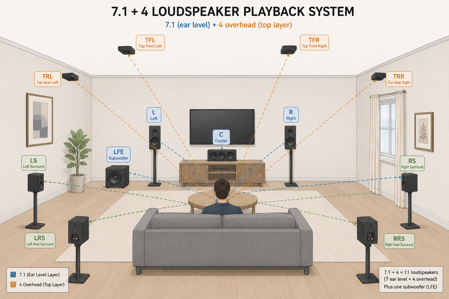
3.5.2 Loudspeaker Layouts
Common loudspeaker array configurations include:
- Stereo: Two loudspeakers (left and right)
- Surround sound: 5.1, 7.1, etc. (standardized layouts)
- Ambisonics: Spherical loudspeaker arrays
- Custom arrays: Arbitrary loudspeaker positions
3.5.3 Panning Laws
To position a virtual source between loudspeakers, we apply panning gains to each loudspeaker. The gains determine how much of the source signal is sent to each loudspeaker.
For a virtual source signal x[n] and loudspeaker gains g_i, the signal sent to loudspeaker i is:
s_i[n] = g_i \cdot x[n] \tag{3.1}
3.5.4 Power-Preserving Panning
To maintain consistent loudness regardless of source position, panning gains should satisfy:
\sum_{i=1}^{N} g_i^2 = \text{constant}
This ensures that the total acoustic power remains constant as the source moves.
3.5.5 Vector Base Amplitude Panning (VBAP)
VBAP is a panning technique that works with arbitrary loudspeaker arrays. It uses a vector-based approach to calculate gains for positioning virtual sources.
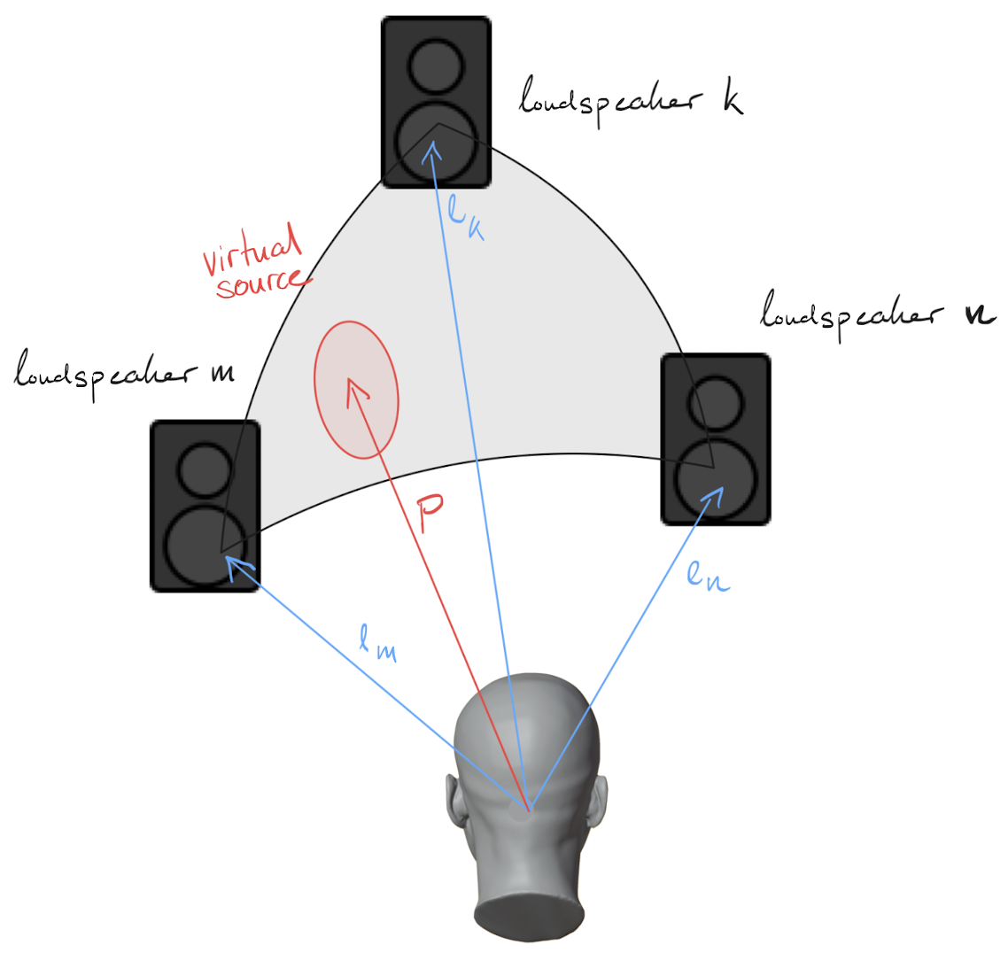
Key principles of VBAP:
- Virtual sources are positioned using a small subset of loudspeakers (typically 2 for 2D, 3 for 3D)
- The active loudspeakers form a “base” (basis vectors)
- Gains are calculated by projecting the source direction onto this base
- Only loudspeakers forming a triangle (or line segment in 2D) containing the source are active
VBAP will be covered in detail in the next section.
3.6 Vector Base Amplitude Panning (VBAP)
3.6.1 Introduction to VBAP
Vector Base Amplitude Panning (VBAP) is a panning technique developed by Ville Pulkki that allows positioning virtual sound sources using arbitrary loudspeaker arrays. VBAP extends traditional stereo panning to 2D and 3D loudspeaker configurations.
3.6.2 Mathematical Foundation
VBAP represents loudspeaker positions as unit vectors \mathbf{l}_i (pointing from the listener to each loudspeaker). A virtual source direction is also represented as a unit vector \mathbf{p}.
The goal is to find gains g_i such that:
\mathbf{p} = \sum_{i=1}^{N} g_i \mathbf{l}_i
where N is the number of active loudspeakers (typically 2 for 2D, 3 for 3D).
3.6.3 Convex Hull and Triangulation
VBAP requires that the loudspeaker array forms a convex hull around the listener:
- Convex hull: The smallest convex shape that contains all loudspeaker positions
- Triangulation: Dividing the convex hull into triangles (2D) or tetrahedra (3D)
- Each triangle/tetrahedron defines a panning region
Why convex hull?:
- Virtual sources can only be positioned within the convex hull
- Sources outside the hull cannot be accurately rendered
- The convex hull defines the sweet spot for the loudspeaker array
3.6.4 Finding Active Loudspeakers
For a given virtual source position \mathbf{p}, VBAP:
- Identifies the containing triangle/tetrahedron: Determines which loudspeakers form the base
- Calculates gains: Solves for the gains that reproduce the source direction
3.6.5 Gain Calculation
For a triangle formed by loudspeakers at positions \mathbf{l}_1, \mathbf{l}_2, \mathbf{l}_3, we solve:
\mathbf{p} = g_1 \mathbf{l}_1 + g_2 \mathbf{l}_2 + g_3 \mathbf{l}_3
In matrix form:
\mathbf{p} = \begin{bmatrix} \mathbf{l}_1 & \mathbf{l}_2 & \mathbf{l}_3 \end{bmatrix} \begin{bmatrix} g_1 \\ g_2 \\ g_3 \end{bmatrix} = \mathbf{L} \mathbf{g}
Solving for gains:
\mathbf{g} = \mathbf{L}^{-1} \mathbf{p}
3.6.6 Gain Constraints
For the source to be within the triangle, all gains must be non-negative:
g_i \geq 0 \quad \forall i
If any gain is negative, the source is outside that triangle, and we must check the next triangle.
3.6.7 Power Normalization
To maintain constant power, gains are normalized:
g_i' = \frac{g_i}{\sum_{j} g_j}
This ensures that the sum of gains equals 1, maintaining consistent loudness.
3.6.8 Implementation Steps
- Compute convex hull: Find the triangulation of the loudspeaker array
- Pre-compute inverse bases: Calculate \mathbf{L}^{-1} for each triangle
- For each virtual source:
- Convert source direction to unit vector
- Find containing triangle (check all triangles until gains are non-negative)
- Calculate gains using inverse base matrix
- Normalize gains
- Apply gains: Multiply source signals by gains and sum to loudspeaker signals
3.6.9 Advantages of VBAP
- Works with arbitrary loudspeaker arrays
- Smooth panning as sources move
- Power-preserving (with normalization)
- Computationally efficient
- Extensible to 3D arrays
3.6.10 Limitations
- Virtual sources must be within the convex hull
- Loudspeaker array must be convex
- May require many loudspeakers for large sweet spots
- Does not account for room acoustics or listener position
3.7 Combined Rendering Pipeline
3.7.1 Combining VBAP and Binaural Rendering
A powerful approach is to combine VBAP and binaural rendering:
- VBAP stage: Position virtual sources using a loudspeaker array (creating “virtual loudspeakers”)
- Binaural stage: Apply HRTFs to the loudspeaker signals to create binaural output
This approach allows:
- Flexible source positioning using VBAP
- Accurate spatialization using individualized or measured HRTFs
- Headphone playback of complex spatial audio scenes
3.7.2 The Complete Pipeline
For a scene with multiple sources:
- Source signals: x_i[n] for sources i = 1, \ldots, N
- VBAP processing: Calculate loudspeaker gains g_{i,j} for source i to loudspeaker j
- Loudspeaker signals: s_j[n] = \sum_{i} g_{i,j} \cdot x_i[n]
- Binaural processing: Apply HRTFs for each loudspeaker direction
- Binaural output: y_L[n] and y_R[n] for headphone playback
3.7.3 Block-Based Processing
For time-varying scenes (moving sources), the pipeline operates block-by-block:
- Update VBAP gains: Recalculate gains for each block based on source positions
- Update HRIRs: Select new HRIRs if loudspeaker directions change
- Process blocks: Apply VBAP and binaural processing to each block
- Smooth transitions: Interpolate gains and HRIRs to avoid artifacts
3.7.4 Applications
This combined approach is used in:
- Virtual reality audio: Rendering complex 3D audio scenes
- Music production: Creating immersive spatial audio mixes
- Gaming: Dynamic spatial audio with moving sources
- Telepresence: Spatial audio for remote collaboration
3.8 Summary and Outlook
3.8.1 Key Concepts Covered
In this handbook, we have introduced the fundamental concepts of spatial audio rendering:
- Binaural hearing: How humans localize sound using ITD, ILD, and spectral cues
- HRTFs and HRIRs: Frequency and time-domain representations of spatial hearing
- Binaural rendering: Convolving source signals with HRIRs to create spatialized audio
- Loudspeaker arrays: Positioning virtual sources using multiple loudspeakers
- VBAP: Vector-based panning technique for arbitrary loudspeaker arrays
- Combined rendering: Using VBAP and binaural rendering together
3.8.2 The Complete Rendering Pipeline
Assignment 2 guides you through implementing:
- HRIR selection: Finding the nearest HRIR for a given source direction
- Binaural processing: Convolving sources with HRIRs using block-based convolution
- Convex hull computation: Triangulating loudspeaker arrays
- VBAP implementation: Calculating gains for virtual source positioning
- Combined rendering: Applying VBAP followed by binaural rendering
3.8.3 Advanced Topics
Beyond Assignment 2, spatial audio rendering includes:
- Ambisonics: Spherical harmonic representation for flexible spatial audio
- Higher-order ambisonics: More accurate spatial audio representation
- Individualized HRTFs: Custom HRTFs for improved localization
- Head tracking: Dynamic HRTF updates based on head orientation
- Distance rendering: Combining spatialization with distance cues
- Room acoustics: Adding early reflections and reverberation to spatial audio