Nonlinear System Identification: Learning a Tanh Distortion System

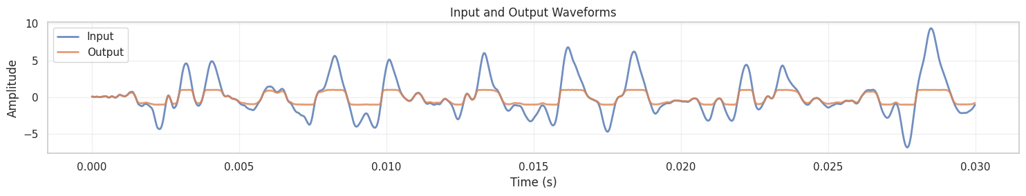
This notebook demonstrates nonlinear system identification using polynomial lifting to learn a nonlinear distortion system. We’ll use real guitar audio as input and a synthetic nonlinear system based on the hype rbolic tangent (tanh) function to create a controlled learning scenario.

Problem Setting

Nonlinear System Identification Block Diagram

The Nonlinear System: Tanh Distortion

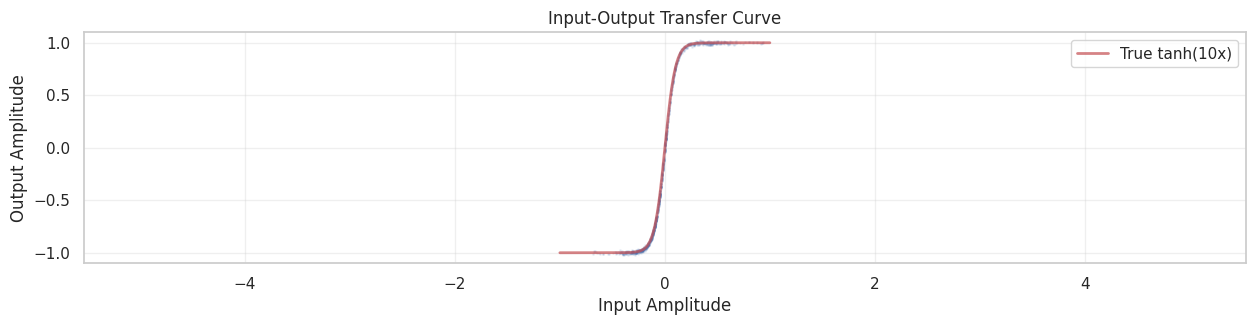
We consider a memoryless nonlinear system that applies a hyperbolic tangent distortion:

y[k] = \tanh(\alpha \cdot x[k]) + n[k]

where:

  • x[k] is the input signal (guitar audio)
  • y[k] is the output signal (distorted audio)
  • \alpha is a gain parameter (we use \alpha = 10 for strong distortion)
  • n[k] is additive noise

Why tanh? The hyperbolic tangent function is commonly used to model:

  • Guitar distortion pedals (fuzz, overdrive effects)
  • Saturation in audio systems (tape saturation, tube amplifiers)
  • Clipping behavior (soft clipping vs hard clipping)

The tanh function has the key property that it saturates for large inputs: as |x| \to \infty, we have |\tanh(x)| \to 1. This creates the characteristic “soft clipping” distortion heard in many guitar effects.

Why Guitar Input?

Guitar signals are ideal for this demonstration because:

  1. Rich harmonic content: Guitar signals contain multiple frequencies that interact through nonlinearity
  2. Dynamic range: Guitar playing naturally varies in amplitude, exercising the nonlinearity across its full range
  3. Musical context: The results are audibly meaningful, making it easier to assess model quality

Learning Objective

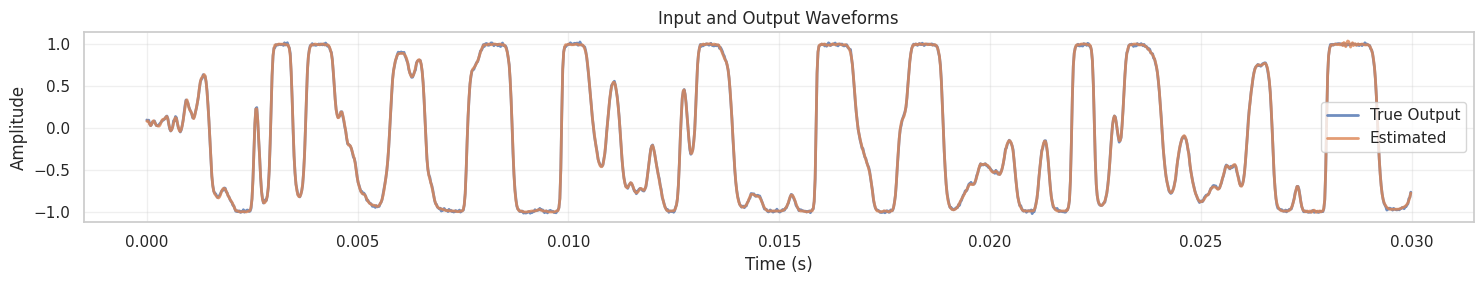
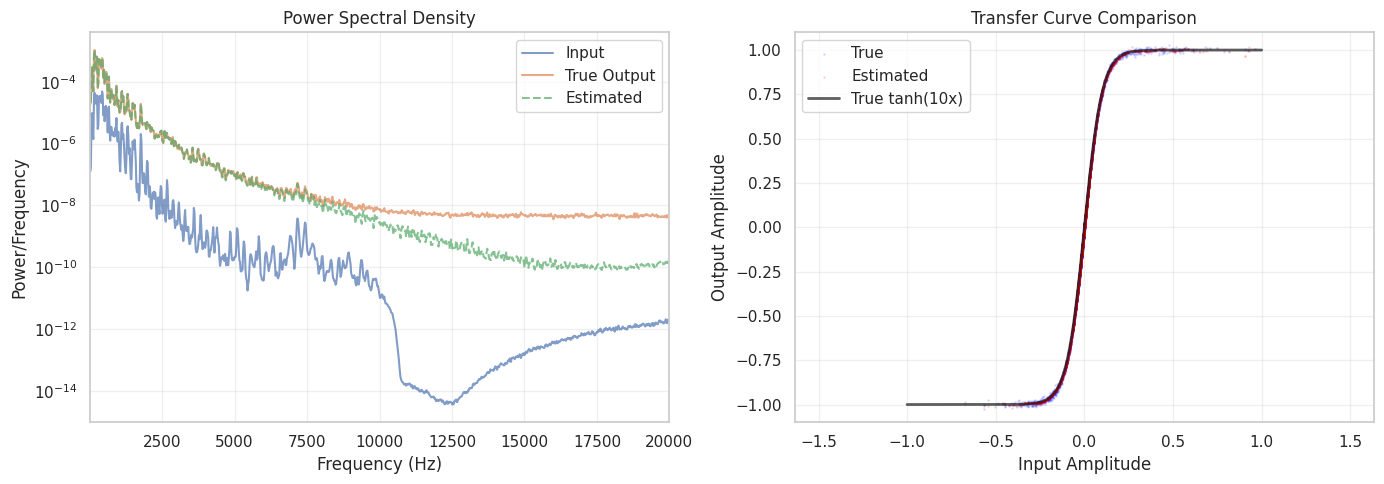
Our goal is to identify the nonlinear system using only input-output pairs (x[k], y[k]) without knowing the underlying tanh function. We’ll use polynomial lifting with Legendre polynomials to approximate the nonlinearity.

Key Concepts We’ll Explore

  1. Polynomial Lifting: Creating a high-dimensional feature space from the input signal
  2. Legendre Polynomials: An orthogonal basis that provides better numerical conditioning than monomials
  3. Least Squares Estimation: Solving for the optimal filter coefficients
  4. Time and Frequency Domain Analysis: Evaluating model performance
Sample rate: 44100 Hz
Duration: 3.73 seconds
Number of samples: 164375

Input Audio (Original Signal $x[k]$):

Output Audio (Nonlinear System Output $y[k]$):

Polynomial Lifting for System Identification

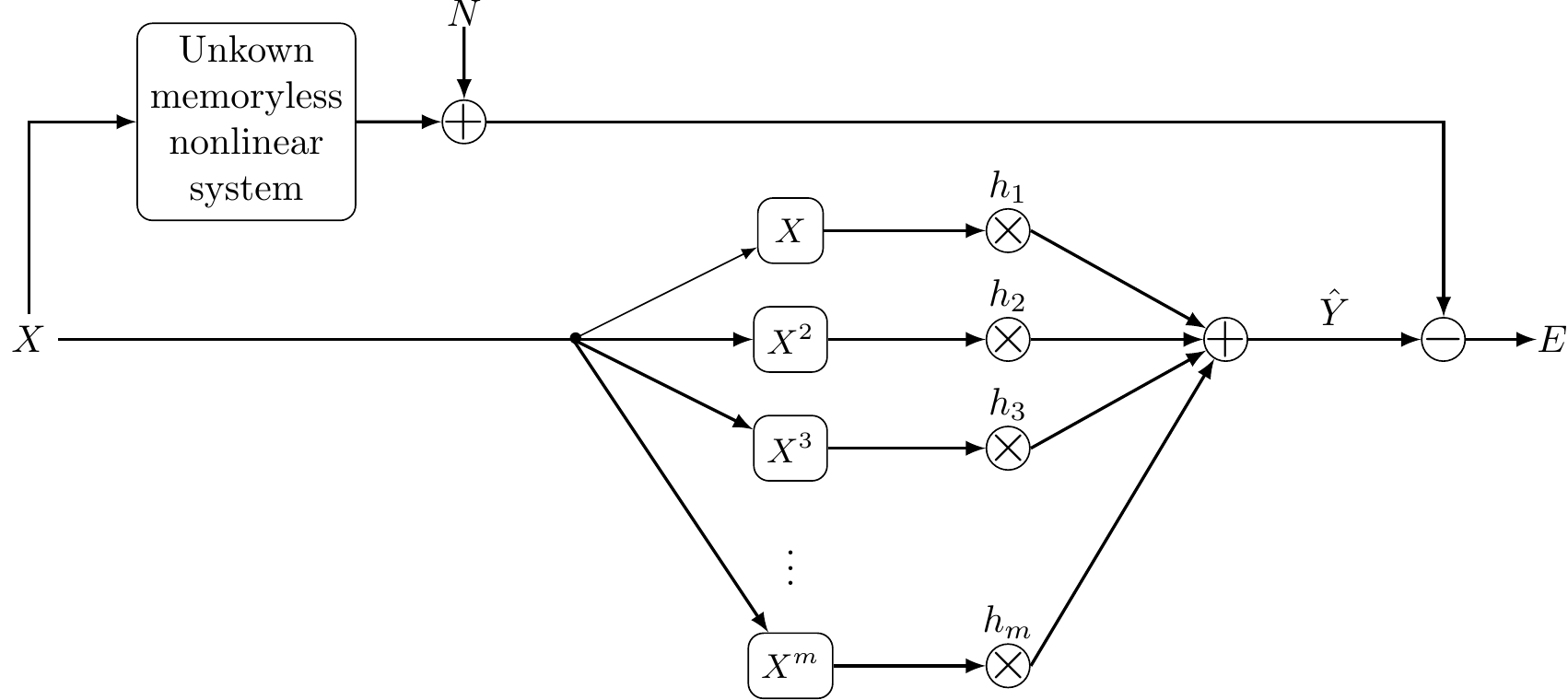
Now we’ll use polynomial lifting to learn the nonlinear system. The key idea is to:

  1. Create a lifted feature space: Transform the input x[k] into a high-dimensional vector \mathbf{z}[k] containing polynomial features
  2. Use Legendre polynomials: These provide an orthogonal basis that is numerically well-conditioned
  3. Solve least squares: Find the optimal linear filter \mathbf{h} that maps features to output

Mathematical Formulation

For a memoryless nonlinear system, we approximate:

\hat{y}[k] = \sum_{m=0}^{M} h_m \cdot x^m[k]

The lifting scheme with the monomials x^m leads to highly correlated features. To avoid this, an alternative lifting scheme is

\hat{y}[k] = \sum_{m=0}^{M} h_m \cdot P_m(x[k])

where P_m(\cdot) are Legendre polynomials of order m, and h_m are the filter coefficients we need to learn.

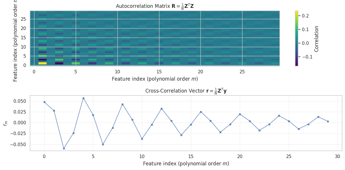
In matrix form, with N samples:

  • Feature matrix: \mathbf{Z} \in \mathbb{R}^{N \times (M+1)} where Z[k,m] = P_m(x[k])
  • Output vector: \mathbf{y} \in \mathbb{R}^{N}
  • Filter vector: \mathbf{h} \in \mathbb{R}^{M+1}

We solve for \mathbf{h} using the normal equation:

\mathbf{R} \mathbf{h} = \mathbf{r}

where:

  • \mathbf{R} = \frac{1}{N}\mathbf{Z}^T\mathbf{Z} is the estimated autocorrelation matrix
  • \mathbf{r} = \frac{1}{N}\mathbf{Z}^T\mathbf{y} is the estimated cross-correlation vector
Training on 150000 samples
Using Legendre polynomials up to order 30

Feature matrix shape: (150000, 30)
Number of features: 30
Autocorrelation matrix shape: (30, 30)
<Figure size 1400x1000 with 0 Axes>


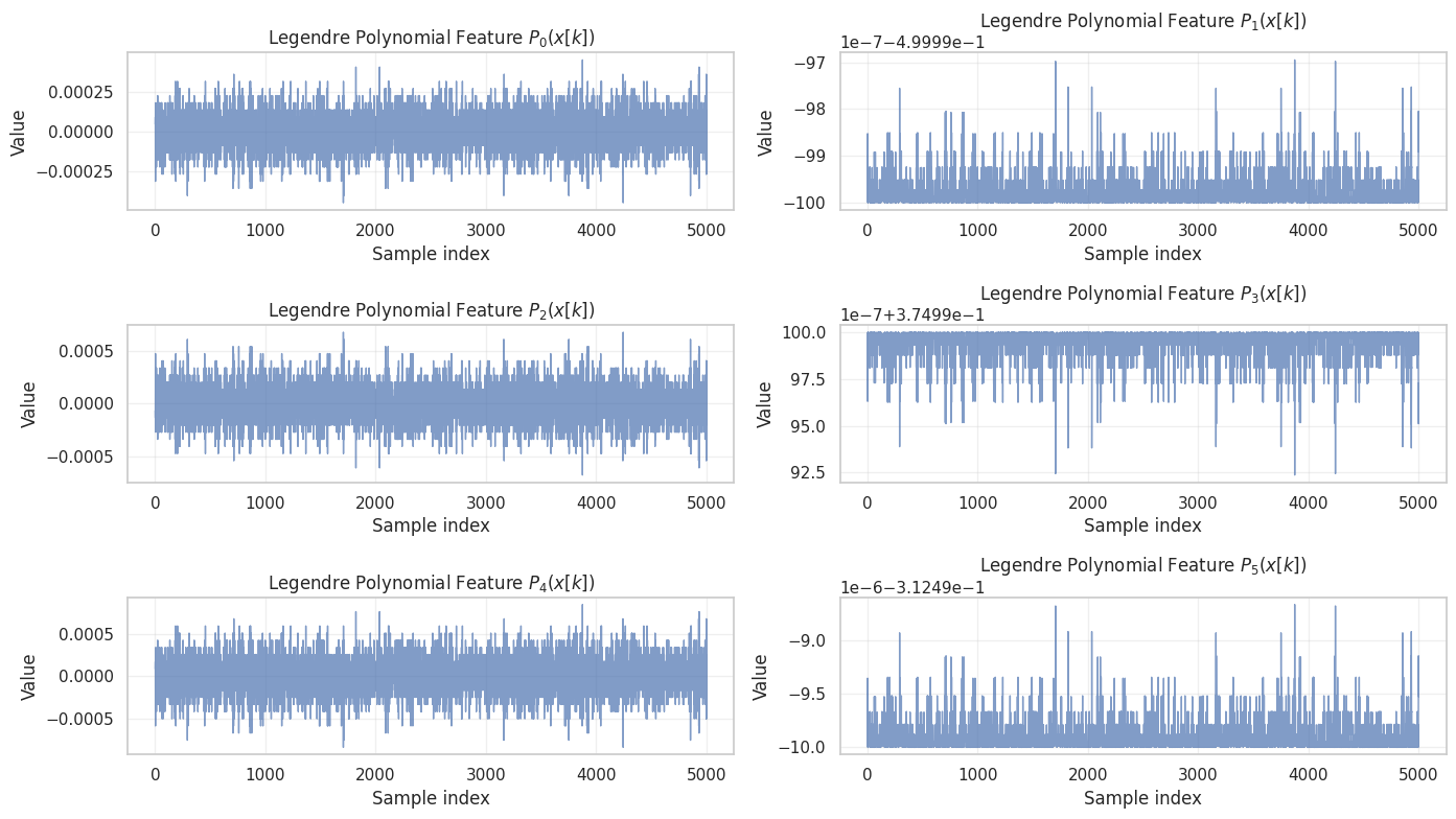
Filter coefficients computed
Total filter parameters: 30
Filter norm: 105.5414


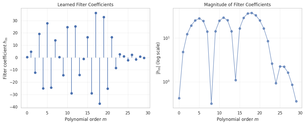
Performance Metrics:
  Mean Squared Error (MSE): 0.000103
  Root Mean Squared Error (RMSE): 0.010160
  Signal-to-Noise Ratio (SNR): 33.42 dB

Input Audio (Original Signal $x[k]$):

Output Audio (Nonlinear System Output $y[k]$):

Estimated Output (Model Estimate $\hat{y}[k]$):