For the maximum likelihood estimation, we require the likelihood of the observations given the estimand. We give examples where this likelihood can be derived from a probabilistic model.
We want to estimate a parameter \theta from multiple observations X_1, X_2, \ldots, X_N, i.e.,
\hat{\theta}_{\text{MLE}} = \arg\max_{\theta} f_{X_1, X_2, \ldots, X_N \mid \theta}(x_1, x_2, \ldots, x_N).
Usually, we assume that the observations are i.i.d., such that
\hat{\theta}_{\text{MLE}} = \arg\max_{\theta} \prod_{i=1}^{N} f_{X \mid \theta}(x_i;\theta) = \arg\max_{\theta} \sum_{i=1}^{N} \log f_{X \mid \theta}(x_i;\theta).
For independent and identically distributed (i.i.d.) samples x_1, x_2, \ldots, x_N from a distribution with parameter \mu, the maximum likelihood estimator maximizes the likelihood function:
\hat{\mu}_{\text{MLE}} = \arg\max_{\mu} \sum_{i=1}^{N} \log f_X(x_i; \mu)
Gaussian Distribution: For X \sim \mathcal{N}(\mu, \sigma^2) with known \sigma^2, the likelihood is f_X(x; \mu) = \frac{1}{\sqrt{2\pi\sigma^2}} \exp\left(-\frac{(x-\mu)^2}{2\sigma^2}\right) such that \log f_X(x_i; \mu) = -\frac{1}{2}\log(2\pi\sigma^2) - \frac{(x_i-\mu)^2}{2\sigma^2}
Taking the derivative with respect to \mu and setting to zero: \frac{\partial}{\partial \mu} \sum_{i=1}^{N} \log f_X(x_i; \mu) = \sum_{i=1}^{N} \frac{x_i-\mu}{\sigma^2} = 0
Solving: \sum_{i=1}^{N} (x_i-\mu) = 0 \Rightarrow N\mu = \sum_{i=1}^{N} x_i
Therefore, the sample mean is the MLE solution \hat{\mu}_{\text{MLE}} = \frac{1}{N}\sum_{i=1}^{N} x_i
Laplacian Distribution: For X \sim \text{Laplace}(\mu, b), likelihood is f_X(x; \mu) = \frac{1}{2b} \exp\left(-\frac{|x-\mu|}{b}\right) such that \log f_X(x_i; \mu) = -\log(2b) - \frac{|x_i-\mu|}{b} .
The MLE for \mu is the value that minimizes \sum_{i=1}^{N} |x_i-\mu|, which is the sample median: \hat{\mu}_{\text{MLE}} = \text{median}(x_1, x_2, \ldots, x_N)
Uniform Distribution: For X \sim \mathcal{U}(a, b) where \mu = (a+b)/2, with the likelihood
f_X(x; a, b) = \begin{cases} \frac{1}{b-a} & \text{if } a \leq x \leq b \\ 0 & \text{otherwise} \end{cases}
The likelihood is constant for all x_i \in [a, b] and zero otherwise. The MLE maximizes the likelihood by making the interval as small as possible while containing all samples: \hat{a}_{\text{MLE}} = \min(x_i), \quad \hat{b}_{\text{MLE}} = \max(x_i)
Therefore, the MLE solution is the sample mid-range \hat{\mu}_{\text{MLE}} = \frac{\hat{a}_{\text{MLE}} + \hat{b}_{\text{MLE}}}{2} = \frac{\min(x_i) + \max(x_i)}{2}
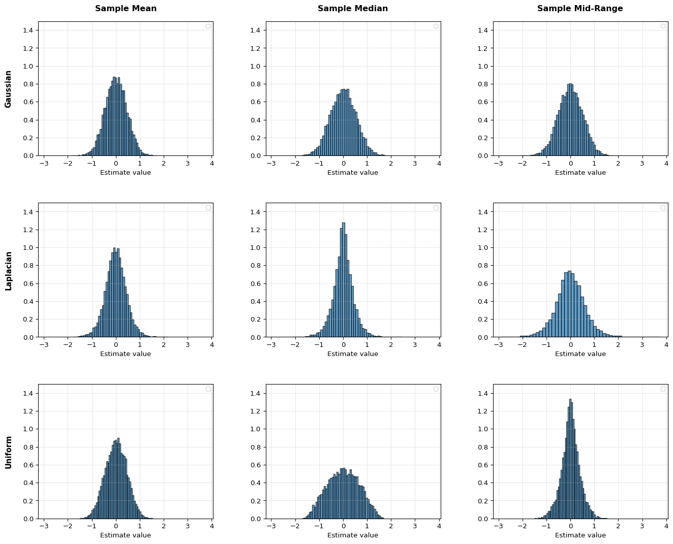
To evaluate the estimators, we can assume a probability distribution X, from which those samples x_i originated. Let’s consider three scenarios: a Gaussian distribution, a Laplacian distribution, and a Uniform distribution, all three with unknown parameters (and their mean).
For our examples, we’ll use:
Let’s take N = 5 samples from those distributions and plot the estimator distributions.
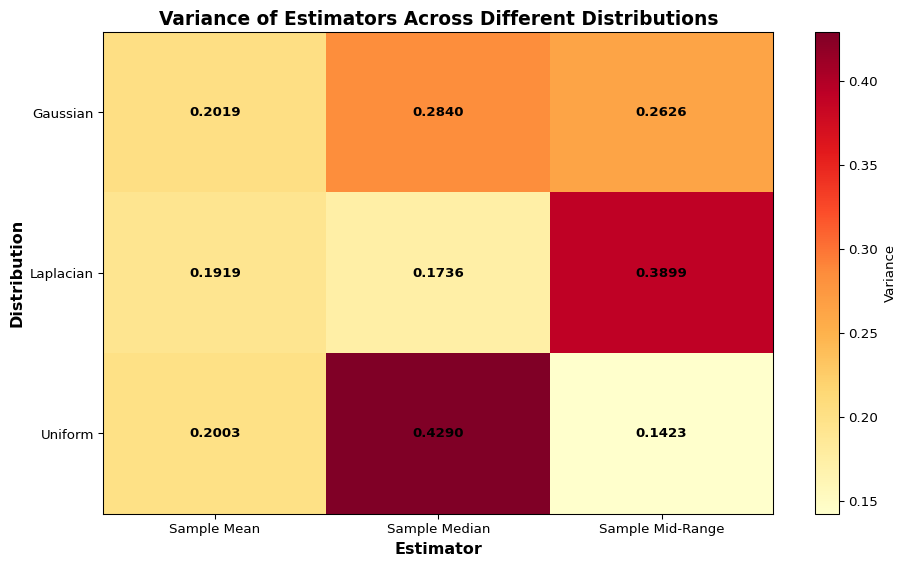
As seen in the graphs, all estimators are unbiased regardless of the distribution as they are symmetric around the true value. However, the variances are vastly different. The sample mean has the same variance across all distributions; however, we see that each distribution has a clearly winning estimator with smallest variance.
Practical note: it is possible to apply any of those estimators to any of the distributions. In the absence of more knowledge, this might be the only practical thing to do. However, this does not guarantee the quality of the estimator.
Probabilistic Model: We assume that the observations follow a linear model with additive noise V:
Y = \mathbf{X}^\top \boldsymbol{\theta} + V.
The likelihood of the parameter \boldsymbol{\theta} given (Y, \mathbf{X}) is
f_{Y \mid \mathbf{X}, \boldsymbol{\theta}}(y \mid \mathbf{x}; \boldsymbol{\theta}) = f_V\left( y - \mathbf{x}^\top \boldsymbol{\theta} \right).
Also, here multiple i.i.d. observations can be combined to a joint likelihood L(\boldsymbol{\theta}) = \prod_{i=1}^{N} f(y_i | \mathbf{x}_i; \boldsymbol{\theta})
We assume Gaussian noise, where v_i \sim \mathcal{N}(0, \sigma^2) are independent and identically distributed (i.i.d.) noise terms. This implies:
y_i \sim \mathcal{N}(\mathbf{x}_i^\top \boldsymbol{\theta}, \sigma^2)
Likelihood Function: For N independent observations \{y_i, \mathbf{x}_i\}_{i=1}^{N}, the likelihood function is:
L(\boldsymbol{\theta}) = \prod_{i=1}^{N} f(y_i | \mathbf{x}_i; \boldsymbol{\theta}) = \prod_{i=1}^{N} \frac{1}{\sqrt{2\pi\sigma^2}} \exp\left(-\frac{(y_i - \mathbf{x}_i^\top \boldsymbol{\theta})^2}{2\sigma^2}\right)
Log-Likelihood: Taking the logarithm:
\ell(\boldsymbol{\theta}) = \log L(\boldsymbol{\theta}) = -\frac{N}{2}\log(2\pi\sigma^2) - \frac{1}{2\sigma^2}\sum_{i=1}^{N} (y_i - \mathbf{x}_i^\top \boldsymbol{\theta})^2
MLE for \boldsymbol{\theta}: To find the MLE of \boldsymbol{\theta}, we maximize the log-likelihood with respect to \boldsymbol{\theta}. Since \sigma^2 > 0 is a constant scaling factor, maximizing \ell(\boldsymbol{\theta}) with respect to \boldsymbol{\theta} is equivalent to minimizing:
\sum_{i=1}^{N} (y_i - \mathbf{x}_i^\top \boldsymbol{\theta})^2
Taking the gradient with respect to \boldsymbol{\theta} and setting to zero:
\nabla_{\boldsymbol{\theta}} \ell(\boldsymbol{\theta}, \sigma^2) = \frac{1}{\sigma^2}\sum_{i=1}^{N} \mathbf{x}_i (y_i - \mathbf{x}_i^\top \boldsymbol{\theta}) = 0
This gives the normal equation:
\left(\sum_{i=1}^{N} \mathbf{x}_i \mathbf{x}_i^\top\right) \hat{\boldsymbol{\theta}}_{\text{MLE}} = \sum_{i=1}^{N} \mathbf{x}_i y_i
In matrix form:
(\mathbf{X}^\top \mathbf{X}) \hat{\boldsymbol{\theta}}_{\text{MLE}} = \mathbf{X}^\top \mathbf{y}
Therefore:
\hat{\boldsymbol{\theta}}_{\text{MLE}} = (\mathbf{X}^\top \mathbf{X})^{-1} \mathbf{X}^\top \mathbf{y}
Key Insight: The MLE estimator under the Gaussian noise assumption is identical to the OLS estimator derived from the empirical risk minimization.
If we change now the probabilistic model, we expect MLE to change as well. Let’s assume Laplacian noise.
Probabilistic Model: We now assume additive Laplacian noise:
y_i = \mathbf{x}_i^\top \boldsymbol{\theta} + v_i
where v_i \sim \text{Laplace}(0, b) are independent and identically distributed (i.i.d.) noise terms with scale parameter b > 0. The probability density function of the Laplacian distribution is:
f_V(v) = \frac{1}{2b} \exp\left(-\frac{|v|}{b}\right)
This implies that y_i has the distribution:
y_i \sim \text{Laplace}(\mathbf{x}_i^\top \boldsymbol{\theta}, b)
with probability density function:
f(y_i | \mathbf{x}_i; \boldsymbol{\theta}) = \frac{1}{2b} \exp\left(-\frac{|y_i - \mathbf{x}_i^\top \boldsymbol{\theta}|}{b}\right)
Likelihood Function: For N independent observations \{y_i, \mathbf{x}_i\}_{i=1}^{N}, the likelihood function is:
L(\boldsymbol{\theta}) = \prod_{i=1}^{N} f(y_i | \mathbf{x}_i; \boldsymbol{\theta}, b) = \prod_{i=1}^{N} \frac{1}{2b} \exp\left(-\frac{|y_i - \mathbf{x}_i^\top \boldsymbol{\theta}|}{b}\right)
Log-Likelihood: Taking the logarithm:
\ell(\boldsymbol{\theta}) = \log L(\boldsymbol{\theta}, b) = -N\log(2b) - \frac{1}{b}\sum_{i=1}^{N} |y_i - \mathbf{x}_i^\top \boldsymbol{\theta}|
MLE for \boldsymbol{\theta}: To find the MLE of \boldsymbol{\theta}, we maximize the log-likelihood with respect to \boldsymbol{\theta}. Since b > 0 is a constant scaling factor, maximizing \ell(\boldsymbol{\theta}, b) with respect to \boldsymbol{\theta} is equivalent to minimizing:
\sum_{i=1}^{N} |y_i - \mathbf{x}_i^\top \boldsymbol{\theta}|
This is the least absolute deviations (LAD) or L1 regression problem, which is different from the least squares (L2) problem!
Key Differences from Gaussian Case:
This numerical example demonstrates the difference between OLS (L2) and LAD (L1) regression under different noise distributions:
The example uses N=15 observations per trial and \sigma_v=1.0 noise level. With Laplacian noise, the heavier tails create outliers where LAD’s robustness shows its advantage over OLS.
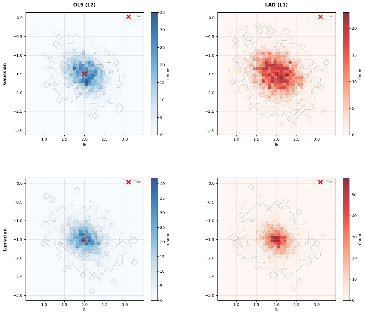
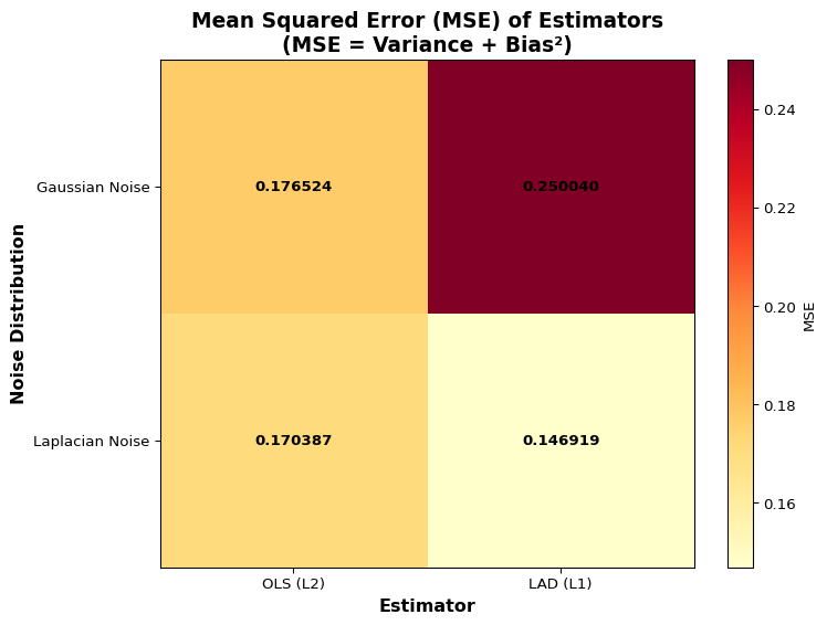
Important Insight: