Linear Transforms of Random Variables

Key Concepts

• Linear Transforms of a Single RV
• Linear Transforms of Random Vectors
• Expectations of Linearly Transformed Random Vectors
• Central Limit Theorem (CLT)

Linear Transforms of Random Vectors

\bf Y = \bf g(\bf X) = {\bf A X}. The pdf is then f_{\bf Y}({\bf y}) = \frac{f_{\bf X}({\bf A}^{-1}{\bf y})} {\left| \textrm{det} {\bf A} \right|}. The moments are {\bf m_Y}= {\bf A} {\bf m_X} \quad, \quad {\bf R}_{\bf YY}= {\bf A}{\bf R}_{\bf XX} {\bf A}^H

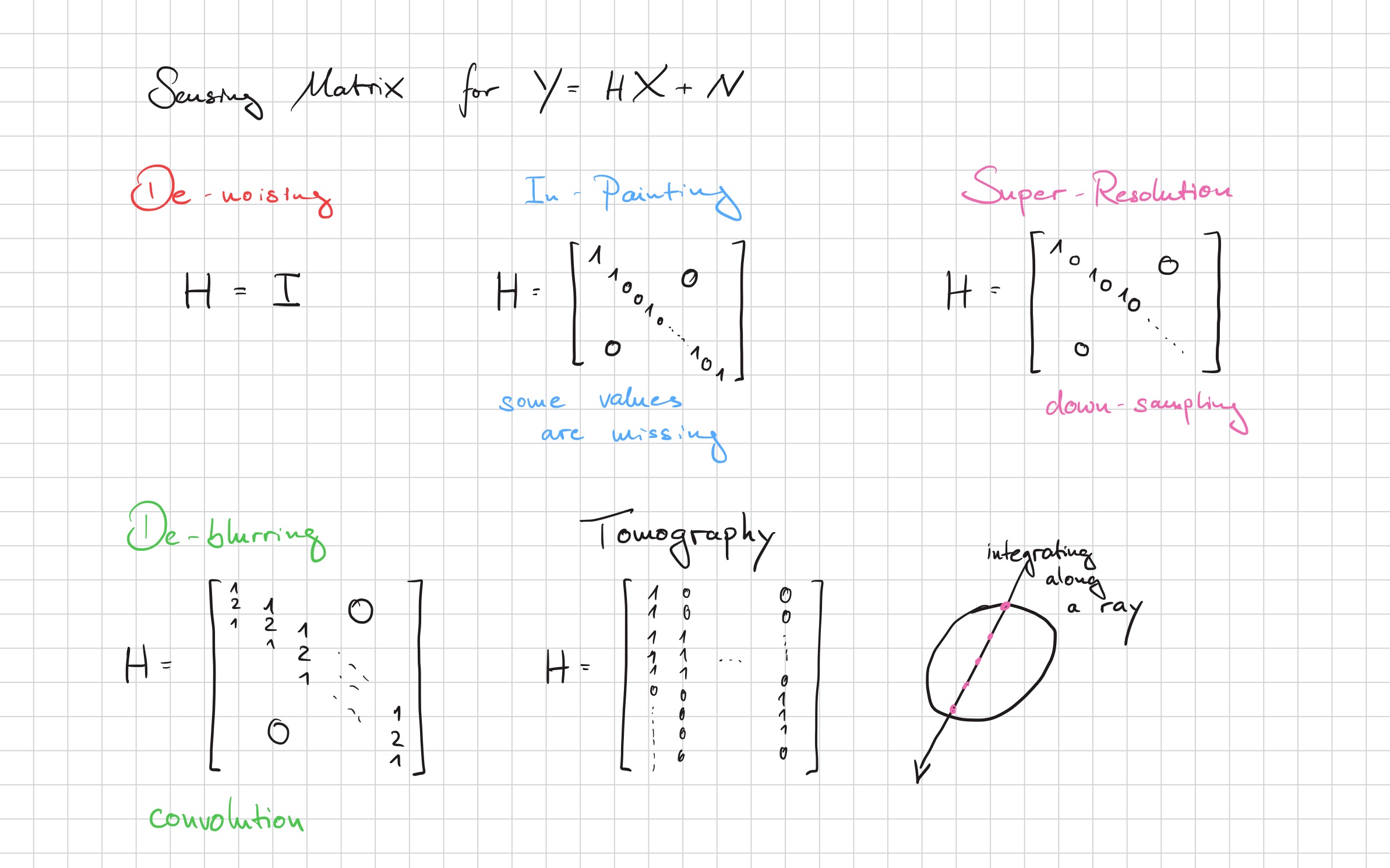
Linear Inverse Problems

Consider a linear model, with the sensing matrix \mathbf{H} and measurement noise \mathbf{N}: \mathbf{Y} = \mathbf{H} \mathbf{X} + \mathbf{N} The inverse problem is to determine \mathbf{X} from measurement \mathbf{Y}, for example, \mathcal{E}\{\mathbf{X} | \mathbf{Y}\}.

De-Noising
In-Painting
Tomography
De-Blurring
De-Mosaicing
Super-Resolution

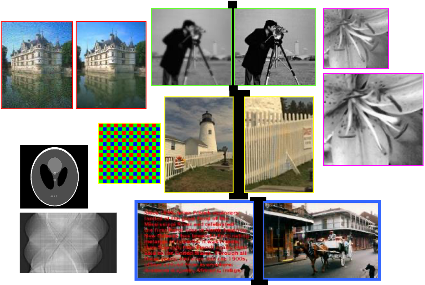
Source: Michael Elad / https://elad.cs.technion.ac.il/

Sensing Matrix

Decorrelation

Choosing \mathbf{A} = \mathbf{Q} as the eigenvectors of \mathbf{R}_{\mathbf{XX}} = \mathbf{Q} \mathbf{\Lambda} \mathbf{Q}^H can decorrelate the RVs. \mathbf{R}_{\mathbf{YY}} = \mathbf{A} \mathbf{R}_{\mathbf{XX}} \mathbf{A}^H = \mathbf{\Lambda}

Central Limit Theorem

Considering now a linear combination of N statistically independent real-valued RVs Y_N =a_1 X_1 + a_2 X_2 + \ldots + a_N X_N := {\bf a}^T {\bf X}, (a_i \neq 0) Under very general conditions, Y tends to approximate a Gaussian distribution. As an example, we chooses X_i to be uniform.