MAP vs MMSE Estimation: Discrete Prior Examples

This notebook demonstrates the conceptual and practical differences between two fundamental Bayesian estimators:

MAP (Maximum A Posteriori): \hat{x}_{\text{MAP}}(y) = \arg\max_i p(x_i \mid y)
MMSE (Minimum Mean Squared Error): \hat{x}_{\text{MMSE}}(y) = \mathcal{E}\{x \mid y\} = \sum_i x_i p(x_i \mid y)

The idea for this demonstration is taken from The Perception-Distortion Tradeoff by Blau and Michaeli.

PART 1 — Small 1D Demonstration

Problem Setup

We start with a simple discrete prior example to build intuition:

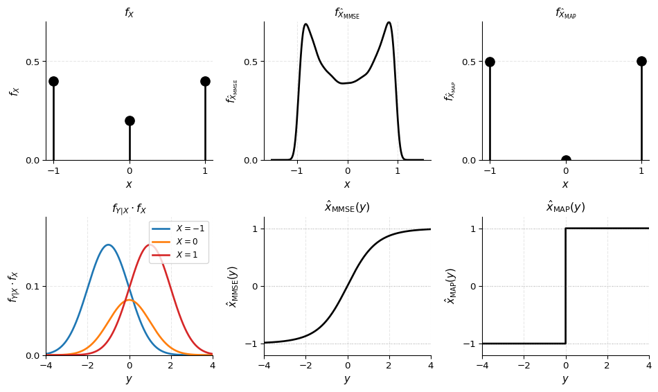
Discrete prior: X \in \{-1, 0, 1\} with probabilities p_X = [0.4, 0.2, 0.4]
Measurement model: Y = X + N where N \sim \mathcal{N}(0, 1)

Given an observation y, we compute:

Posterior: f(x_i \mid y) \propto f(y \mid x_i) f(x_i)
MAP estimator: Selects the single most probable dictionary element \hat{x}_{\text{MAP}}(y) = \arg\max_x f(x \mid y)
MMSE estimator: Computes the weighted average of all dictionary elements, weighted by their posterior probabilities \hat{x}_{\text{MMSE}}(y) = \mathcal{E}\{X \mid Y=y\} = \sum_i x_i f(x_i \mid y)

Likelihood and Posterior

The likelihood of observing y given candidate x_i is:

f(y \mid x_i) \propto \exp\left( -\frac{\|y - x_i\|^2}{2\sigma^2} \right)

Resulting Estimator

Summary: Why MAP and MMSE Differ

Key Observations:

MAP estimator is piecewise constant: \hat{x}_{\text{MAP}}(y) takes discrete values \{-1, 0, 1\} and jumps between them as y crosses decision boundaries. This is because MAP selects the single most probable value from the discrete set.
MMSE estimator is smooth: \hat{x}_{\text{MMSE}}(y) is a continuous, smooth function of y because it computes the weighted average \sum_i x_i p(x_i \mid y). As y changes, the posterior probabilities change smoothly, leading to a smooth estimate.
Distribution differences:
- The MAP estimate distribution is discrete (only takes values \{-1, 0, 1\}) and differs from the prior because MAP selects based on the posterior, which depends on the observation y.
- The MMSE estimate distribution is continuous and centered around the prior mean, but with reduced variance (it’s a “shrunk” version of the prior).
Why MMSE is smoother: MMSE integrates over uncertainty by averaging all candidates weighted by their posterior probability. MAP ignores this uncertainty and picks only the mode, leading to discrete jumps.

This simple 1D example illustrates the fundamental difference: MAP selects a single discrete candidate, while MMSE computes a weighted average, resulting in smooth, continuous estimates even when the prior is discrete.

PART 2 — MNIST Image Denoising Example

Problem Setup

We now apply the same concepts to a high-dimensional image denoising problem using MNIST images.

Likelihood and Posterior

The likelihood of observing y given candidate image x_i is:

f(y \mid x_i) \propto \exp\left( -\frac{\|y - x_i\|^2}{2\sigma^2} \right)

The posterior over the discrete set is:

p(x_i \mid y) \propto p(y \mid x_i) p(x_i)

where p(x_i) is the prior probability of image x_i (uniform in our main experiment).

1. Load MNIST Data

We’ll download MNIST and normalize pixel values to [0, 1]. Images will be flattened for computation but we’ll keep a reshape helper for visualization.

Training images shape: (60000, 784)
Test images shape: (10000, 784)
Pixel value range: [0.000, 1.000]

2. Select Test Image and Add Noise

We’ll pick a test image and add Gaussian white noise to create our noisy observation y.

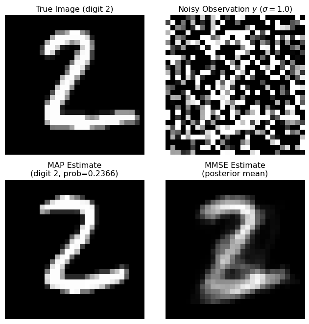
Selected test image: digit 2
Noise standard deviation: 1.0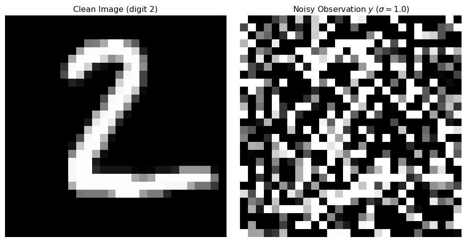

3. Build Discrete Prior Dictionary

We’ll use the first N_CANDIDATES training images as our dictionary \{x_1, \dots, x_N\}. This approximates a continuous prior by a finite set of candidate images. We assume a uniform prior over these images.

Dictionary size: 4000 images
Dictionary shape: (4000, 784)
Prior: Uniform

4. Compute Log-Likelihoods and Posterior Probabilities

Log-Likelihood Function

The log-likelihood is:

\log p(y \mid x_i) = -\frac{\|y - x_i\|^2}{2\sigma^2} + \text{constant}

We can ignore the constant term since it cancels out when normalizing the posterior.

Numerical Stability

For numerical stability, we work entirely in the log-domain and use the log-sum-exp trick to normalize probabilities:

\log p(x_i \mid y) = \log p(y \mid x_i) + \log p(x_i) - \log Z

where Z = \sum_j \exp(\log p(y \mid x_j) + \log p(x_j)) is the normalization constant.

Sum of posterior probabilities: 1.000000
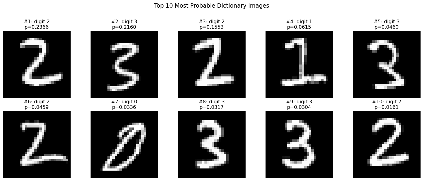
Max posterior probability: 0.236598
Min posterior probability: 8.227841e-16
Number of non-negligible probabilities (>1e-6): 758

5. MAP Estimator

The MAP estimator selects the single most probable dictionary element:

\hat{x}_{\text{MAP}}(y) = \arg\max_i p(x_i \mid y)

This is equivalent to finding the index with maximum unnormalized log-posterior (since log is monotonic).

Key insight: MAP picks the single “best match” from the dictionary. If the true image is in the dictionary and noise is not too large, MAP will likely pick it or something visually very similar.

MAP estimate: dictionary index 1609
MAP posterior probability: 0.236598
MAP digit label: 2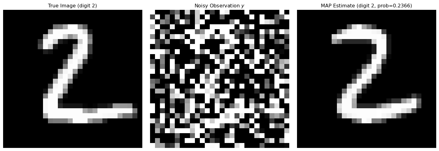

6. MMSE Estimator

The MMSE estimator computes the posterior mean:

\hat{x}_{\text{MMSE}}(y) = \mathbb{E}[x \mid y] = \sum_i x_i p(x_i \mid y)

Key insight: MMSE averages over all candidate images weighted by their posterior probabilities. This often produces a smoother, more “blurred” result because it integrates over multiple plausible candidates, not just the single most probable one.

MMSE estimate computed as weighted average over 4000 images
Effective number of images (exp entropy): 13.30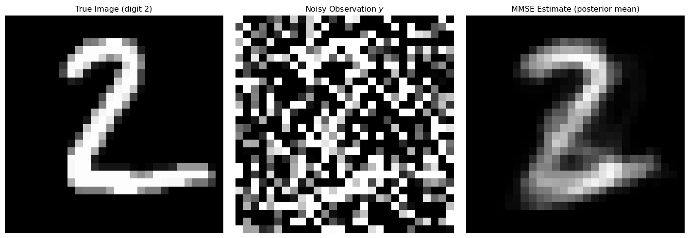

7. Visualize Posterior Structure

Let’s examine the top K most probable dictionary images according to the posterior. This helps us understand:

MAP picks only the top-1 image (the single most probable)
MMSE integrates over the full posterior, including all of these top candidates

The MMSE estimate is a weighted average of these (and many other) images.

8. Direct Comparison: MAP vs MMSE

Let’s create a clean comparison figure showing both estimators side-by-side.

Qualitative Differences

MAP Estimator:

Picks the single most probable dictionary element
Often produces sharper results (since it’s a single clean image)
Can be “wrong” in a structured way if the true image isn’t in the dictionary
Computationally simpler (just find argmax)

MMSE Estimator:

Computes the weighted average over all dictionary elements
Often appears smoother/blurrier because it averages multiple plausible candidates
Optimal in the MSE sense (minimizes expected squared error)
Can produce “ghost” images that blend features from multiple digits

The key difference is that MAP selects a single discrete candidate, while MMSE integrates over the entire posterior distribution, producing a continuous-valued estimate that may not correspond to any single dictionary element.

9. MSE Comparison

Let’s compute the pixel-wise Mean Squared Error (MSE) for each estimator to quantitatively compare their performance.

Mean Squared Error (MSE) Comparison:
  Noisy observation y:     MSE = 0.264886
  MAP estimate:           MSE = 0.047396
  MMSE estimate:          MSE = 0.045642

Improvement over noisy:
  MAP:  82.1% reduction
  MMSE: 82.8% reduction

MMSE vs MAP:
  MMSE has lower MSE (as expected, by 3.7%)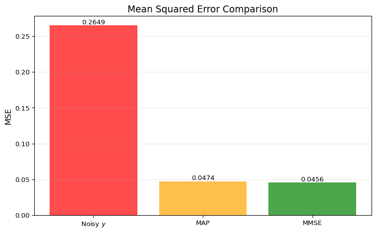

Why MMSE Minimizes Expected MSE

The MMSE estimator \hat{x}_{\text{MMSE}} = \mathbb{E}[x \mid y] minimizes the expected squared error:

\mathbb{E}[\|x - \hat{x}\|^2 \mid y]

This is a fundamental result in Bayesian estimation theory. For any specific realization, MAP might occasionally achieve lower MSE, but on average (over many realizations), MMSE will have the lowest MSE.

In our discrete setting, MMSE computes the posterior mean, which is the optimal estimator under the squared error loss function.

10. Optional: True Image Not in Dictionary

Let’s explore what happens when the true image is not in the dictionary. We’ll create a modified test image (e.g., by masking part of it) and see how MAP and MMSE behave differently.

Modified test image (top half masked out)
This image is NOT in the dictionary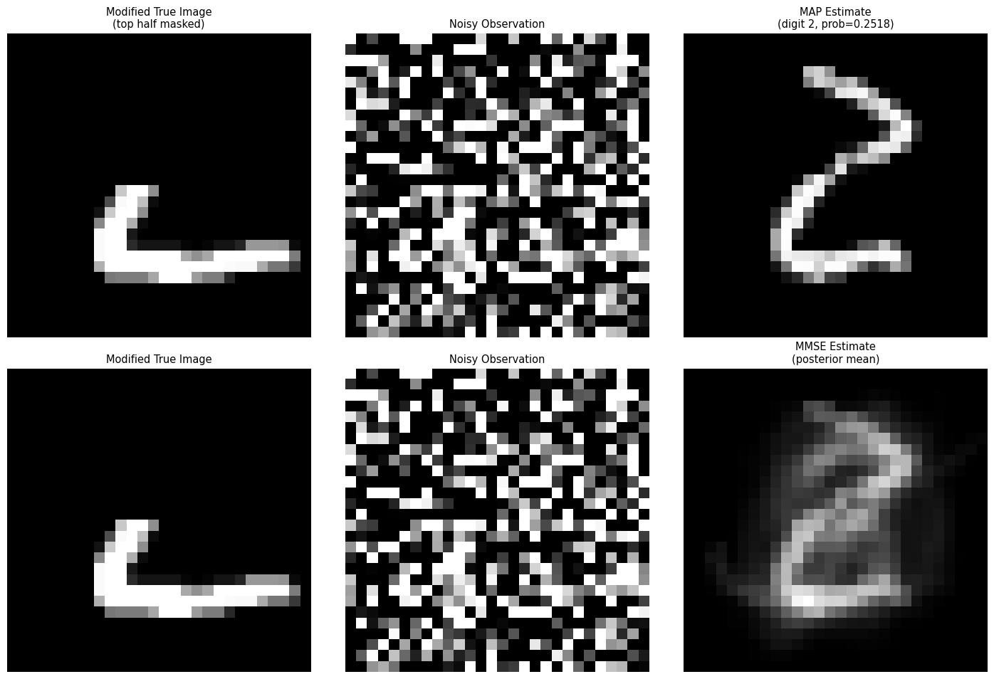


MSE for modified image:
  MAP:  0.055568
  MMSE: 0.047006

Discussion: When True Signal is Outside Prior Support

When the true image is not in the dictionary (outside the support of the prior):

MAP picks the single “closest” digit from the dictionary, which may be visually similar but structurally different
MMSE produces an average of multiple similar digits, which can create a “blended” or “ghost” image that doesn’t correspond to any single digit

This illustrates an important limitation: both estimators are constrained by the dictionary. If the true signal space is much richer than the dictionary, the estimates will be biased toward the dictionary elements.

In practice, this motivates:

Using larger, more diverse dictionaries
Using continuous priors (e.g., generative models) instead of discrete dictionaries
Understanding the trade-off between computational tractability and representational power