Expected Values

Key Concepts

• Expectation and Linearity
• Moments (Mean, Variance, Skewness, Kurtosis)
• Conditional Expectations
• Joint Moments of Real-valued RVs
• Correlation, Orthogonality and Independence
• Moments of Real-valued Random Vectors
• Moments of Complex-valued Random Variables and Vectors
• Properties of (Auto)Correlation Matrices
• Correlation Matrices of Random Processes

Moments of random variables

The probability of extreme events

Independence and Correlation

Statistical independence does imply zero correlation. However, the reverse is not true.

Let X be a zero-mean, symmetric random variable, and define Y = X^2. Then:

\mathcal{E}\{X\} = 0, \qquad \mathcal{E}\{Y\} = \mathcal{E}\{X^2\} = \sigma_X^2, \qquad \mathcal{E}\{XY\} = \mathcal{E}\{X^3\} = 0

Hence, X and Y are uncorrelated because \mathrm{C}_{XY} = \mathcal{E}\{XY\} - \mathcal{E}\{X\}\mathcal{E}\{Y\} = 0,

They are clearly not independent, because knowing Y tells you the magnitude of X.

Correlation matrix of vectors

The (auto)correlation matrix of a random vector {\bf X} is given by {\bf R}_{\bf XX} = {\cal E}\left\{{\bf X}{\bf X}^T \right\}.

The centralized version is the (auto)covariance matrix with mean vector {\bf m_X} = {\cal E}\{{\bf X}\}: {\bf C}_{\bf XX} = {\cal E}\left\{({\bf X} - {\bf m_X})({\bf X} - {\bf m_X})^T \right\} = {\bf R}_{\bf XX} - {\bf m_X}{\bf m_X}^T,

The correlation coefficient matrix is obtained by normalizing the covariance matrix with respect to the marginal standard deviations: {\bf \rho}_{\bf XX} = {\bf D}_{\bf X}^{-1/2}\, {\bf C}_{\bf XX}\, {\bf D}_{\bf X}^{-1/2}, where {\bf D}_{\bf X} = \mathrm{diag}({\bf C}_{\bf XX}) contains the variances of the individual components.

Estimated Moments

In practice, the true expectations are unknown and must be estimated from data samples {\bf x}^{(1)}, {\bf x}^{(2)}, \dots, {\bf x}^{(M)}. The sample mean and sample covariance matrix are given by: \widehat{\bf m}_X = \frac{1}{M} \sum_{m=1}^M {\bf x}^{(m)}, \qquad \widehat{\bf C}_{\bf XX} = \frac{1}{M-1} \sum_{m=1}^M ({\bf x}^{(m)} - \widehat{\bf m}_X)({\bf x}^{(m)} - \widehat{\bf m}_X)^T.

From this, the sample normalized covariance matrix is \widehat{\bf \rho}_{\bf XX} = {\bf D}_{\widehat{\bf X}}^{-1/2}\, \widehat{\bf C}_{\bf XX}\, {\bf D}_{\widehat{\bf X}}^{-1/2}. where \widehat{\bf D}_{\bf X} = \mathrm{diag}(\widehat{\bf C}_{\bf XX}) contains the variances of the individual components.

Student Performance Data

We visualize the joint distribution and estimate the covariance matrix using data from a student exam performance dataset (Kaggle source).

Each data samples contain three values: \mathbf{x}^{(i)}= [‘Hours Studied’, ‘Attendance %’, ‘Exam Score’].

Student Performance Data - Covariance

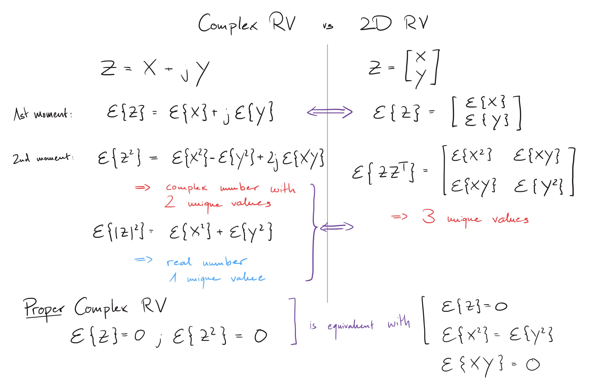
Moments of a complex-valued random variable

Complex random variables can be represented in two ways: Z(\eta) = X(\eta) + j Y(\eta) = R(\eta) \cdot \exp (j \Phi(\eta))

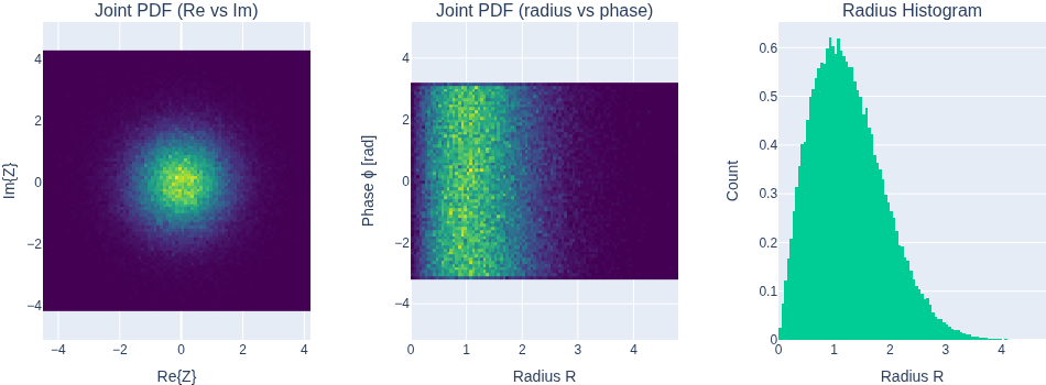
For a complex random variable with independent radius and phase, the moments are m_Z^{(n)} = \mathcal{E}[R^{n}] \mathcal{E}[e^{j\Phi n}] For a uniform phase \Phi \sim U[0,2\pi], all the moments are zero.

The absolute moment is however m_Z^{|n|} = \mathcal{E}\{|Z|^{n}\} = \mathcal{E}\{R^{n}\}

Complex Random Variables vs 2D Random Variables

Complex RV vs 2D RV

Radially symmetric complex Gaussian

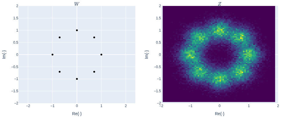
Phase-shift-keying (PSK) and additive noise

The phase shift key is modeled by Z = W + N, where W = \exp(jK) with K \sim U[0,1,\dots,M-1] and N as complex-valued noise, for example, Gaussian.

Application: Eigenfaces

A more advanced application of expected values are shown in the Eigenface Demo