AR(1) process generated with a = 0.9Innovation
Wold Decomposition
For any zero-mean, stationary process X[k], the Wold decomposition states:
X[k] = X^{\text{det}}[k] + X^{\text{stoch}}[k],
Deterministic Component
X^{\text{det}}[k] is perfectly predictable:
- Finite sum of sinusoids or exact periodic component
- Autocorrelation sequence is periodic
- No innovation: \varepsilon[k] = X^{\text{det}}[k] - \widehat{X}^{\text{det}}[k|k-1] = 0
Periodic autocorrelation \Rightarrow deterministic component
Stochastic Component
X^{\text{stoch}}[k] is noise-driven:
- absolutely summable impulse response,
- non-periodic autocorrelation (“regular part”),
- a representation X^{\text{stoch}}[k]=\sum_{i=0}^\infty h_i W[k-i], where W[k] is white (the innovation).
Regular autocorrelation \Rightarrow stochastic component
Autocorrelation Decomposition
Let the autocorrelation be split as:
R_x[m] = R_{\textrm{reg}}[m] + R_{\textrm{per}}[m] .
- R_{\text{per}}[m]: periodic (harmonic) → deterministic harmonics
- R_{\text{reg}}[m]: “regular” → the part that has a spectral factor → stochastic
Innovation
A process W[k] is a (weak) innovation for a process X[k] if:
W[k] is (weakly) white: \mathbb{E}\{W[k+1]W[n]\} = 0, \quad n \leq k.
W[k+1] is orthogonal to the past of X: W[k+1] \perp \text{span}\{X[n]: n \leq k\}.
Here, \text{span}\{X[n]: n \leq k\} denotes the set of all linear combinations of the random variables \{X[n]: n \leq k\}, i.e., all random variables of the form \sum_{j \leq k} a_j X[j] for some coefficients a_j.
Interpretation
The innovation W[k+1] represents the “new information” in X[k+1] that cannot be predicted from the past values \{X[n]: n \leq k\}. Since W[k+1] is orthogonal to all linear combinations of past X values, it captures the part of X[k+1] that is uncorrelated with and unpredictable from its history. This makes innovations fundamental for prediction, filtering, and understanding the information content of stochastic processes.
Innovation Representation
We assume:
W[k] is (weakly) white: \mathbb{E}\{W[k+1]W[n]\} = 0, \quad n \leq k.
X and W are related by a causal, stable, minimum-phase filter h and its inverse: X = h * W, \qquad W = h_{\text{inv}} * X, with both h and h_{\text{inv}} causal and stable.
From causality we get:
- X[j] depends only on \{W[n]: n \leq j\},
- W[j] depends only on \{X[n]: n \leq j\}.
Thus
\overline{\text{span}\{X[n] : n \leq k\}} = \overline{\text{span}\{W[n] : n \leq k\}}
as closed linear subspaces in the L^2 sense.
This equality of subspaces is what minimum-phase of the filter h buys you.
Orthogonality Argument
Now take any linear combination of past X: Y_k = \sum_{j \leq k} a_j X[j].
Because of the causal/invertible relationship, this Y can also be written purely in terms of past W: Y_k = \sum_{n \leq k} b_n W[n] for some coefficients b_n (this is exactly what the inverse filtering does).
Then \mathbb{E}\{W[k+1] Y_k\} = \mathbb{E}\left\{W[k+1]\sum_{n \leq k} b_n W[n]\right\} = \sum_{n \leq k} b_n\, \mathbb{E}\{W[k+1] W[n]\} = 0, because W is white and all indices n in the sum satisfy n \leq k.
Since this holds for any linear combination Y_k of past X’s, we have
W[k+1] \perp \text{span}\{X[n]: n \leq k\},
i.e., W[k+1] is orthogonal to the entire past of X. That is exactly the (weak) innovations property.
Example: AR(1) Process
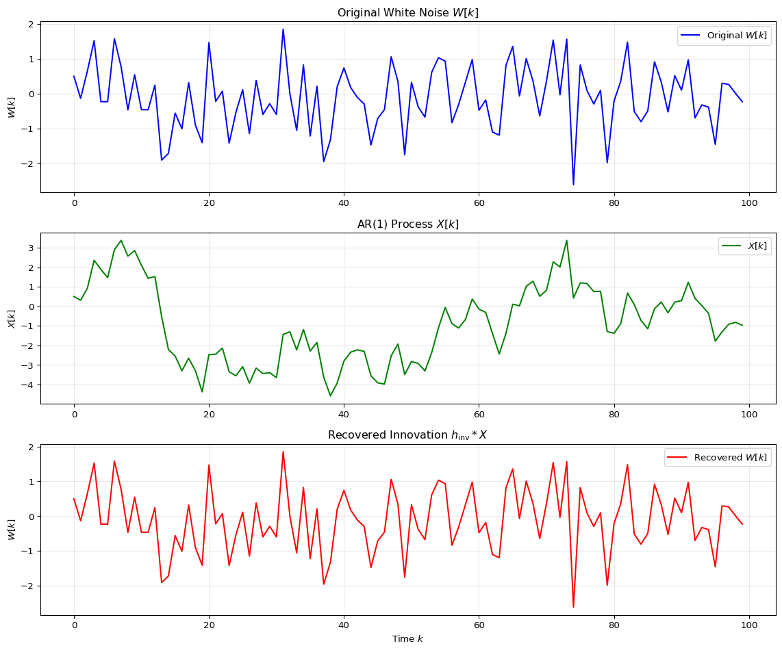
Consider an AR(1) process defined by: X[k] = a X[k-1] + W[k], where |a| < 1 for stability, and W[k] is a white noise process with variance \sigma_W^2.
This can be written as X = h * W where h is the impulse response of the filter. The filter h and its inverse h_{\text{inv}} can be derived from the AR(1) difference equation.
Filter Synthesis
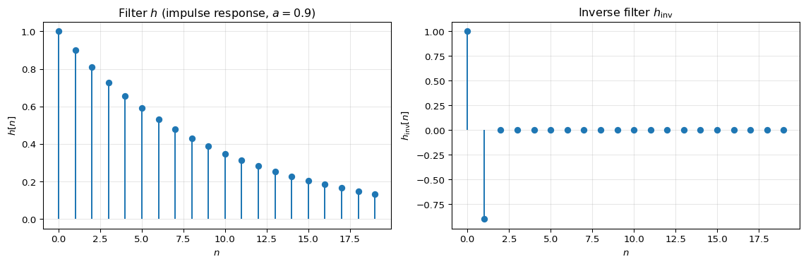
For the AR(1) process X[k] = a X[k-1] + W[k], we can write it in the z-domain as: X(z) = \frac{1}{1 - a z^{-1}} W(z) = H(z) W(z), where H(z) = \frac{1}{1 - a z^{-1}} is the transfer function.
The impulse response h[n] is: h[n] = a^n u[n], where u[n] is the unit step function (i.e., h[n] = 0 for n < 0 and h[n] = a^n for n \geq 0).
The inverse filter h_{\text{inv}} satisfies h_{\text{inv}} * h = \delta, which gives: h_{\text{inv}}[n] = \delta[n] - a \delta[n-1], i.e., h_{\text{inv}}[0] = 1, h_{\text{inv}}[1] = -a, and h_{\text{inv}}[n] = 0 otherwise.
Analysis filter
We verify that applying the inverse filter to X recovers the innovation W: W = h_{\text{inv}} * X.
Spectral Factorization via Cepstral Analysis
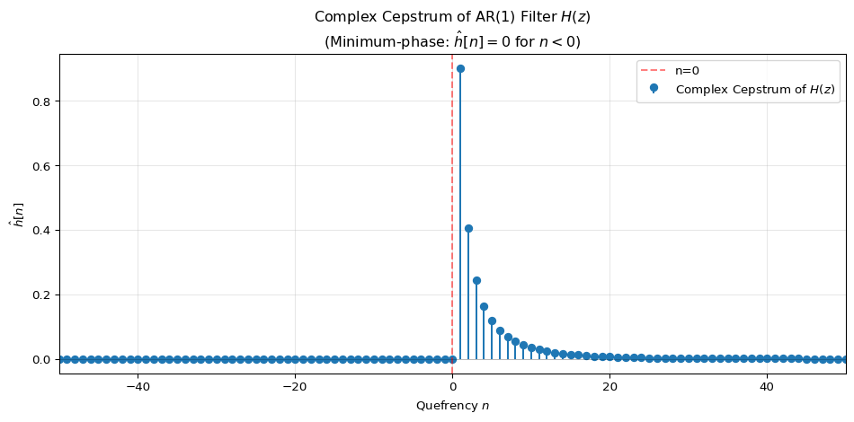
Cepstrum of a Minimum-Phase Filter
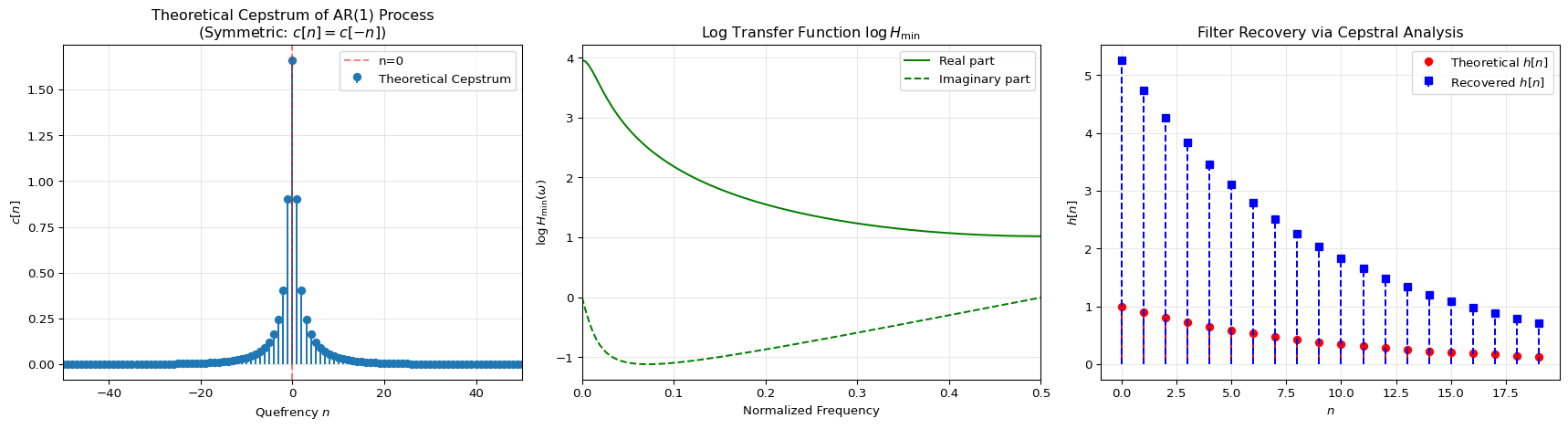
For a minimum-phase filter H(z), the complex cepstrum (cepstrum of H(\omega)) is causal: \hat{h}[n] = \mathcal{F}^{-1}\{\log H(\omega)\}, where \hat{h}[n] = 0 for n < 0. This causal property is what characterizes minimum-phase systems.
For the AR(1) filter H(z) = \frac{1}{1 - a z^{-1}}, the complex cepstrum is: \hat{h}[0] = 0, \hat{h}[n] = \frac{a^n}{n}, \quad n > 0, \hat{h}[n] = 0, \quad n < 0.
Spectral factorization
Spectral factorization is the process of decomposing a power spectral density (PSD) into a minimum-phase filter and its complex conjugate. For the AR(1) process, we can use cepstral analysis to recover the filter h from the power spectrum.
The cepstrum is defined as the inverse Fourier transform of the logarithm of the power spectrum: c[n] = \mathcal{F}^{-1}\{\log S_X(\omega)\}, where S_X(\omega) is the power spectral density of X[k].
Since S_X(\omega) = \sigma_W^2 |H(\omega)|^2 = \sigma_W^2 H(\omega) H^*(\omega), we have \log S_X(\omega) = \log(\sigma_W^2) + \log H(\omega) + \log H^*(\omega), which means the cepstrum of the power spectrum splits additively: c[n] = \log(\sigma_W^2)\delta[n] + \hat{h}[n] + \hat{h}^*[-n], where \hat{h}[n] is the complex cepstrum of H(\omega) (causal for minimum-phase) and \hat{h}^*[-n] is the complex cepstrum of H^*(\omega) (anti-causal).
Cepstrum for AR(1)
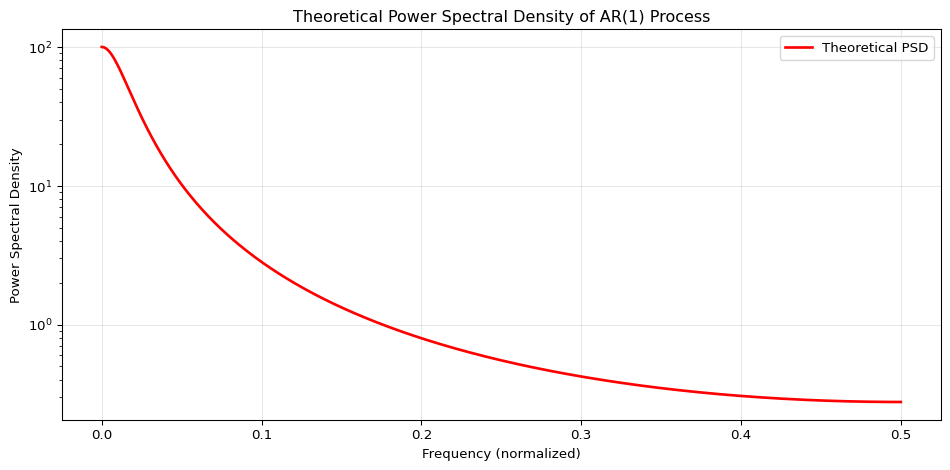
For an AR(1) process, the cepstrum can be computed analytically. The power spectral density is: S_X(\omega) = \frac{\sigma_W^2}{|1 - a e^{-j\omega}|^2} = \frac{\sigma_W^2}{1 - 2a\cos(\omega) + a^2}.
Since the power spectral density is real and even, its inverse Fourier transform (the cepstrum) must also be real and even, i.e., symmetric: c[n] = c[-n].
Taking the logarithm and computing the inverse Fourier transform, the theoretical cepstrum coefficients for AR(1) are: c[0] = \log\left(\frac{\sigma_W^2}{1 - a^2}\right), c[n] = \frac{a^{|n|}}{|n|}, \quad n \neq 0.
The cepstrum decays exponentially with |n|, reflecting the fact that the AR(1) process has a single pole at z = a. For minimum-phase reconstruction, we extract only the causal part (n \geq 0) of this symmetric cepstrum.