Statistical Signal Processing - Multichannel Filtering

Linear Sensor Array for Acoustic Spatial Filtering

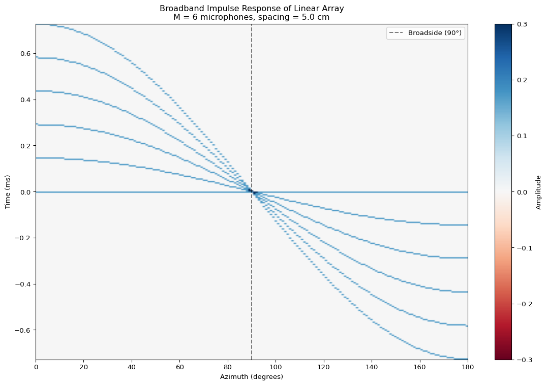
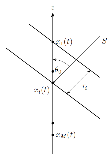
Linear Array A linear sensor array consists of M sensors (microphones) arranged vertically in a straight line with uniform spacing d between adjacent sensors. When a plane wave impinges on the array from direction \theta_0 (measured from horizontal, where 90° is broadside, i.e., perpendicular to the vertical array), each sensor receives the signal with a different time delay.

Time Delays

For a linear array, the time delay \tau_i at sensor i relative to the reference sensor (i=1) is:

\tau_i = \frac{d_i \cdot \sin(\theta_0)}{c},

where:

• i = 1, 2, \ldots, M is the sensor index
• d_i is the relative distance from the reference sensor to sensor i (in meters)
• \theta_0 is the direction of arrival (DOA) angle
• c is the speed of sound (approximately 343 m/s)

The reference sensor (i=1) serves as the reference, so \tau_1 = 0. For a wave arriving from broadside (\theta_0 = 90°), all sensors receive the signal simultaneously. For waves arriving from other angles, the delays create a phase progression across the array that can be exploited for spatial filtering.

Delay-and-Sum Beamforming

The simplest spatial filtering approach is to sum all sensor signals with appropriate delays to align signals from a desired direction. This is called delay-and-sum beamforming.

If we simply sum the sensor outputs each with their propagation delay, the signals from a plane wave at angle \theta_0 are:

y(t) = \sum_{i=1}^{M} x_i\left(t\right) = \sum_{i=1}^{M} s\left(t - \tau_i\right)

where s(t) is the source signal, x_i(t) is the signal received at microphone i and \tau_i is the physical propagation delay to sensor i for a wave arriving at angle \theta_0.

The corresponding impulse response is h(t; \theta_0) = \sum_{i=1}^{M} \delta\left( t - \tau_i \right) .

This creates a spatial filter that:

• Coherently adds signals from directions where \cos(\theta_0) results in constructive interference
• Attenuates signals from other directions due to destructive interference

Frequency Response vs Azimuth

The magnitude frequency response of the delay-and-sum beamformer shows how the array responds to signals from different directions at different frequencies. The response is strongest when signals add coherently (in phase), which occurs at specific angles depending on frequency.

The transfer function H(\omega, \theta) of the delay-and-sum array for a given azimuth \theta is the Fourier Transform of the array’s broadband impulse response h(t, \theta):

H(\omega, \theta) = \int_{-\infty}^{\infty} h(t, \theta)\, e^{-j\omega t}\,dt = \sum_{i=1}^{M} e^{-j\omega \tau_i}

For our sampled impulse responses, this is computed using the discrete Fourier Transform (DFT) of each direction’s response.

Key observations:

• The response is strongest at broadside (90^\circ), where signals coherently combine at all frequencies.
• Spatial aliasing occurs above approximately 6kHz making the array unable to resolve angles accurately.
• At low frequencies, the array is not very selective (broad beam).
• At higher (but sub-aliasing) frequencies, the main lobe is narrower, and directivity improves.

Optimum Multichannel Filtering

MMSE-optimum Linear Multichannel Filtering

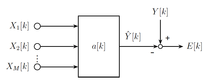
We consider a MISO system (e.g., an array of sensors) whose input signals should be linearly combined to form a linear MMSE estimate.

\widehat{Y}[k] = \mathbf{a}^H[k] \mathbf{X}[k]

The linear MMSE solution is \mathbf{a}_{\text{MMSE}}[k] = \mathbf{R}_{\mathbf{XX}}^{-1}[k] r_{\mathbf{X}Y}[k]

Linearly Constrained Minimum Variance (LCMV)

Often the reference signal Y[k] is not directly observable. Instead we use constraint to make the problem solvable: \mathbf{C}^H \mathbf{a} = \mathbf{g} and minimize the variance of \widehat{Y} which is \mathbf{a}^H[k] \mathbf{R}_{\mathbf{XX}} \mathbf{a}. This results in (without the time-dependency) \mathbf{a}_{\text{LCMV}} = \mathbf{R}_{\mathbf{XX}}^{-1} \mathbf{C} (\mathbf{C}^H \mathbf{R}_{\mathbf{XX}}^{-1} \mathbf{C})^{-1} \mathbf{g}

Spatial filtering with LCMV

Linear Array Considering a linear sensor array with propagation delay \tau_i to the reference sensor with a plane waves impinging. The source signal S is narrowband around \omega_0. The steering vector depending on direction of arrival (DOA) \theta_0 is \mathbf{d(\theta)} = [e^{j\omega_0 \tau_1}, e^{j\omega_0 \tau_2}, \ldots, e^{j\omega_0 \tau_M}] = [1, e^{j\omega_0 \tau_2}, \ldots, e^{j\omega_0 \tau_M}] where \tau_1 = 0 since sensor i=1 serves as the reference. Constraints can be \text{distortionless: } \mathbf{d(\theta_0)}^H \mathbf{a} = 1 \text{supression: } \mathbf{d(\theta_1)}^H \mathbf{a} = 0

Spatial Filtering Scenario

Consider a scene with one source signal (speaker) at \theta_0 and two interferer at \theta_1 and \theta_2. Listen to the mixture of the sounds in one microphone. The goal is to surpress the interferers.

Sound sources: Interferers and Speech

Mixture at microphone 1:

Estimating the Correlation Matrix

The microphone signals X are source signals \mathbf{S} filtered by steering vectors \mathbf{D} and the sensor noise \mathbf{N}: \mathbf{X}[\omega,n] = \mathbf{D}(\omega) \mathbf{S}[\omega,n] + \mathbf{N}[\omega,n] The correlation matrix is then \mathbf{R}_{\mathbf{XX}}[\omega] = \underbrace{\mathbf{D}(\omega)\mathbf{R}_{\mathbf{SS}}(\omega)\mathbf{D}^H(\omega)}_{\text{Signal + Interference}} + \underbrace{\sigma^2\mathbf{I}}_{\text{Noise}} The correlation matrix is estimated by averaging in the STFT domain. \widehat{\mathbf{R}}_{\mathbf{XX}}[\omega] = \frac{1}{N_{\text{frames}}} \sum_{n=1}^{N_{\text{frames}}} \mathbf{X}[\omega, n] \mathbf{X}^H[\omega, n]

Microphone 1 (Input)

LCMV Output

MVDR

MVDR minimizes output variance while maintaining unit gain toward the desired direction \theta_0: \min_{\mathbf{a}} \mathbf{a}^H \mathbf{R}_{\mathbf{XX}} \mathbf{a} \quad \text{subject to} \quad \mathbf{d}^H(\theta_0) \mathbf{a} = 1 Solution: \mathbf{a}_{\text{MVDR}} = \frac{\mathbf{R}_{\mathbf{XX}}^{-1} \mathbf{d}(\theta_0)}{\mathbf{d}^H(\theta_0) \mathbf{R}_{\mathbf{XX}}^{-1} \mathbf{d}(\theta_0)}

Microphone 1 (Input)

MVDR Output

Spatial Filtering Analysis

The response response of the beamformers can be computed by B(\theta, \omega) = \left|\mathbf{a}^H[\omega] \mathbf{d}(\theta, \omega)\right|^2

Source Localization with MVDR

The MVDR beamformer can be used for direction-of-arrival (DOA) estimation by scanning across all angles and finding peaks in the output power.

The MVDR spatial spectrum is the expected output power: P_{\text{MVDR}}(\theta, \omega) = \mathbf{a}_{\text{MVDR}}(\omega)^H \mathbf{R}_{\mathbf{XX}}(\omega) \mathbf{a}_{\text{MVDR}}(\omega) = \frac{1}{\mathbf{d}^H(\theta, \omega) \mathbf{R}_{\mathbf{XX}}^{-1}[\omega] \mathbf{d}(\theta, \omega)}

The peaks of the MVDR spectrum correspond to the source locations.